Session 3

Visualisation and validation of the LSP metrics derived from S2 and Fused Time Series

In this tutorial we show the visualization of the result of the LSP retrieval for maize fields in Brandenburg in 2022, in comparison to the DWD reference and HR-VPP European products.

Input:

• LPS metrics (SoS, PoS, EoS) derived from S2 and Fused NDVI time series
• References (DWD, HR-VPP)

• Outputs:

• csv files with the extracted SoS, PoS, EoS from our analysis and references
• Comparison of violin plots for SoS, PoS, EoS
• Box-plots with the data density impact on phenometrics accuracy

Steps:

1. Global settings
2. Reading and extracting SoS, PoS, EoS from HR-VPP products and from our analysis outputs for selected maize fields
3. Visualisation of violin plots of LSP
4. Error metrics calculation (RSME, MAE, Bias)
5. Error metrics differences per phenometric
6. Box plot comparison of error metrics - Improvement through Fused dataset vs S2

1. Global settings and Python framework

import pandas as pd
import geopandas as gpd
import numpy as np
import rasterio
from rasterio.mask import mask
import matplotlib.pyplot as plt
import seaborn as sns
import os
from matplotlib.colors import ListedColormap
from datetime import datetime
%matplotlib inline
from PIL import Image
from PIL.ExifTags import TAGS
from osgeo import gdal
from pathlib import Path

2. Extract phenometrics values (DOY) from multiple tiffs and save to the csv files

HR-VPP references

### Extraction of DOY values from HR-VPP products. The raster files need to be in WGS UTM 33

shapefile_path = './References/IACS/2022_fid13_maize_subset.shp'

raster_paths = ['./References/VPP/VPP_2022_S2_T33UUT-010m_V105_s1_SOSD_utm.tif',
                './References/VPP/VPP_2022_S2_T33UUT-010m_V105_s1_EOSD_utm.tif',
                './References/VPP/VPP_2022_S2_T33UUT-010m_V105_s1_MAXD_utm.tif'
               ]

# Read the shapefile (fields)
polygons = gpd.read_file(shapefile_path)

# Function to extract values from a raster file within polygons
def extract_values(raster_path, polygons):
    with rasterio.open(raster_path) as src:
        values_list = []
        for _, polygon in polygons.iterrows():
            geom = polygon.geometry
            masked_data, _ = mask(src, [geom], crop=True)
            values = masked_data.flatten()
            values = values[(values > 22000) & (values < 23000)] # the value is related to the year (22) and doy (000)
            values_list.append(values)
    return values_list

# Create a dictionary to store values for each raster
all_values = {}

# Create an empty DataFrame
df = pd.DataFrame()

# Iterate over raster paths
for raster_path in raster_paths:
    raster_name = Path(raster_path).stem  # Extracting the name without extension
    print(f"Processing raster: {raster_name}")

    values_list = extract_values(raster_path, polygons)

    ## Subtract 22000 for year 2022 from each value
    adjusted_values_list = [[value - 22000 for value in values] for values in values_list] # -21000 mean only for year 2021

    # Flatten the adjusted values list
    flattened_values = [value for adjusted_values in adjusted_values_list for value in adjusted_values]

    # Debugging statements
    print(f"Number of polygons: {len(polygons)}")
    print(f"Number of value lists extracted: {len(values_list)}")
    print(f"Total number of adjusted values: {len(flattened_values)}")

    # Add the flattened adjusted values to the DataFrame
    df[raster_name + '_adjusted'] = pd.Series(flattened_values)

# Save the DataFrame to a CSV file
csv_path = './VPP_pheno_2022_vpp_orig-22000.csv'
df.to_csv(csv_path, index=False)

print(f"DONE: Pixel values within the polygons from multiple rasters have been saved to {csv_path}")

S2-based LSP outputs

# Extraction of LSP DOY values from S2-based retrieval methods.

main_directory = './LSP_outputs/S2_2022_0.05_output_v1/'

# Function to list all TIFF files in the specified directories
def list_tiff_files(main_directory):
    tiff_files = []
    for dirpath, _, filenames in os.walk(main_directory):
        for filename in filenames:
            if filename.endswith('.tif'):
                tiff_files.append(os.path.join(dirpath, filename))
    return tiff_files

# List all TIFF files in the main directory
raster_paths = list_tiff_files(main_directory)

# Read the shapefile (polygons)
polygons = gpd.read_file(shapefile_path)

# Function to extract values from a raster file within polygons
def extract_values(raster_path, polygons):
    with rasterio.open(raster_path) as src:
        values_list = []
        for _, polygon in polygons.iterrows():
            geom = polygon.geometry
            masked_data, _ = mask(src, [geom], crop=True)
            values = masked_data.flatten()
            values = values[values != 0]
            values_list.append(values)
    return values_list

# Iterate over raster paths and extract values for each raster
all_values = {}
for raster_path in raster_paths:
    raster_name = Path(raster_path).stem  # Extracting the name without extension
    values_list = extract_values(raster_path, polygons)
    all_values[raster_name] = [value for values in values_list for value in values]

# Create a DataFrame with extracted values
df = pd.DataFrame(all_values)

# Save the DataFrame to a CSV file
#csv_path = './S2_pheno_2022.csv'
csv_path = './S2_pheno_2022.csv'
df.to_csv(csv_path, index=False)

print(f"DONE: Pixel values within the polygons from multiple rasters have been saved to {csv_path}")

Fused-based LSP outputs

# Extraction of LSP DOY values from Fused-based retrieval methods.
main_directory = './LSP_outputs/Fused_2022_0.05_output_v1/'

# Function to list all TIFF files in the specified directories
def list_tiff_files(main_directory):
    tiff_files = []
    for dirpath, _, filenames in os.walk(main_directory):
        for filename in filenames:
            if filename.endswith('.tif'):
                tiff_files.append(os.path.join(dirpath, filename))
    return tiff_files

# List all TIFF files in the main directory
raster_paths = list_tiff_files(main_directory)

# Read the shapefile (polygons)
polygons = gpd.read_file(shapefile_path)

# Function to extract values from a raster file within polygons
def extract_values(raster_path, polygons):
    with rasterio.open(raster_path) as src:
        values_list = []
        for _, polygon in polygons.iterrows():
            geom = polygon.geometry
            masked_data, _ = mask(src, [geom], crop=True)
            values = masked_data.flatten()
            values = values[values != 0]
            values_list.append(values)
    return values_list

# Iterate over raster paths and extract values for each raster
all_values = {}
for raster_path in raster_paths:
    raster_name = Path(raster_path).stem  # Extracting the name without extension
    values_list = extract_values(raster_path, polygons)
    all_values[raster_name] = [value for values in values_list for value in values]

# Create a DataFrame with extracted values
df = pd.DataFrame(all_values)

# Save the DataFrame to a CSV file
csv_path = './Fused_pheno_2022.csv'
df.to_csv(csv_path, index=False)

print(f"DONE: Pixel values within the polygons from multiple rasters have been saved to {csv_path}")

3. Violin plots of LSP

# DWD references for 2022

########### DWD For SoS
# DWD fixed value for phase 67 (beginning of shooting)
specific_value67 = 153
# DWD fixed value for phase 12 (emergence)
specific_value12 = 127

########## DWD For EoS
# DWD fixed value for phase 20 (dough ripening)
specific_value20 = 230
# DWD fixed value for phase 24 (harvest)
specific_value24 = 250

########## DWD For PoS (tip of tassel emergence)
specific_value65 = 187

# Read data from the CSV files
df_m1 = pd.read_csv('./S2_pheno_2022.csv', sep=',')
df_m2 = pd.read_csv('./Fused_pheno_2022.csv', sep=',')
df_m3 = pd.read_csv('./VPP_pheno_2022_vpp_orig-22000.csv', sep=',')

Comparing SOS vs DWD and HR-VPP

# Plotting SoS vs DWD and VPP reference

# Select parameters and methods for plotting
params_to_plot1 = [
   'S2_sos_2022_median_of_slope',
    'S2_sos_2022_relative_amplitude_mean']

params_to_plot2 = [
    'Fused_sos_2022_median_of_slope',
    'Fused_sos_2022_relative_amplitude_mean']

params_to_plot3 = ['VPP_2022_S2_T33UUT-010m_V105_s1_SOSD_utm_adjusted']

# Combine selected parameters from all datasets
df_combined = pd.concat([df_m1[params_to_plot1], df_m2[params_to_plot2], df_m3[params_to_plot3]],  axis=1)

# Reshape DataFrame for Seaborn's violin plot
df_melted = pd.melt(df_combined, value_vars=params_to_plot1 + params_to_plot2 + params_to_plot3)

# Set up the plot
plt.figure(figsize=(12, 6))

# Calculate median values for each parameter
medians = df_combined.median()

# DWD fixed value for phase 67 (beginning of shooting)
plt.axvline(x=specific_value67, color='green', linestyle='dashed', linewidth=1, label=f'Specific Value: {specific_value67}')
# Add text to the line with vertical rotation
plt.text(specific_value67, len(params_to_plot1 + params_to_plot2 + params_to_plot3) + 0.8, f'DWD Shooting:\n{specific_value67}', rotation=45,
          ha='center', verticalalignment='bottom', color='green', fontsize=12)

# DWD fixed value for phase 12 (emergence)
plt.axvline(x=specific_value12, color='brown', linestyle='dashed', linewidth=1, label=f'Specific Value: {specific_value12}')
# Add text to the line with vertical rotation
plt.text(specific_value12, len(params_to_plot1 + params_to_plot2 + params_to_plot3) + 0.8, f'DWD Emergence:\n{specific_value12}', rotation=45,
          ha='center', verticalalignment='bottom', color='brown', fontsize=12)

# Create a horizontal violin plot with strip plot
sns.violinplot(x='value', y='variable', data=df_melted, inner="quartile", split=True, orient='h', palette='Set2', legend=False, hue='variable')

# Display median values on the right axis with vertical offset
horizontal_offset = -15  # Adjust this value as needed
vertical_offset = 0.25  

for i, (param, median) in enumerate(medians.items()):
    plt.text(median - horizontal_offset, i + vertical_offset, f'Median: {median:.2f}', ha='left', va='center', color='brown', fontsize=12)

# Count non-NaN entries in each parameter column
s2_count = df_m1[params_to_plot1[0]].count()
fused_count = df_m2[params_to_plot2[0]].count()
vpp_count = df_m3[params_to_plot3[0]].count()

# Create the annotation text with data counts
counts_text = f"S2: {s2_count}\nFused: {fused_count}\nVPP: {vpp_count}"

# Add the text box to the plot
plt.text(0.02, 0.97, counts_text, fontsize=9, transform=plt.gca().transAxes,
         verticalalignment='top', color='black', bbox=dict(facecolor='white', alpha=0.6))

# Customize the plot
plt.title('SoS - 2022 - ndvi - bspline 0.05 fitting vs VPP and DWD', fontsize=14)
plt.xlabel('DOY', fontsize=14)
plt.ylabel('SoS Retrieval method', fontsize=14)
plt.tick_params(axis='both', which='major', labelsize=14)
plt.yticks(range(len(params_to_plot1 + params_to_plot2 + params_to_plot3)), 
           [
            'S2_SoS-median',  
            'S2_SoS-relative_mean',
            'Fused_SoS-median', 
            'Fused_SoS-relative_mean', 
            'VPP_SoS'])
# Show the plot
plt.show()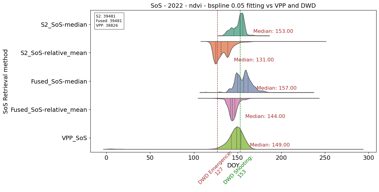

Comparing EOS vs DWD and HR-VPP

# Plotting EoS vs DWD and VPP reference

params_to_plot1 = [
    'S2_eos_2022_median_of_slope',
    'S2_eos_2022_relative_amplitude_mean'
    ]

params_to_plot2 = [
    'Fused_eos_2022_median_of_slope',
    'Fused_eos_2022_relative_amplitude_mean'
    ]

params_to_plot3 = ['VPP_2022_S2_T33UUT-010m_V105_s1_EOSD_utm_adjusted']

# Combine selected parameters from all datasets
df_combined = pd.concat([df_m1[params_to_plot1], df_m2[params_to_plot2], df_m3[params_to_plot3]],  axis=1)

# Reshape DataFrame for Seaborn's violin plot
df_melted = pd.melt(df_combined, value_vars=params_to_plot1 + params_to_plot2 + params_to_plot3)

# Set up the plot
plt.figure(figsize=(12, 6))

# Calculate median values for each parameter
medians = df_combined.median()

# DWD fixed value for phase 20 (dough ripening)
plt.axvline(x=specific_value20, color='orange', linestyle='dashed', linewidth=1, label=f'Specific Value: {specific_value20}')

# Add text to the line with vertical rotation
plt.text(specific_value20, len(params_to_plot1 + params_to_plot2 + params_to_plot3) + 0.8, f'DWD D.Ripening:\n{specific_value20}', rotation=45,
          ha='center', verticalalignment='bottom', color='orange', fontsize=12)

# DWD fixed value for phase 24 (harvest)
plt.axvline(x=specific_value24, color='brown', linestyle='dashed', linewidth=1, label=f'Specific Value: {specific_value24}')

# Add text to the line with vertical rotation
plt.text(specific_value24, len(params_to_plot1 + params_to_plot2 + params_to_plot3) + 0.7, f'DWD Harvest:\n{specific_value24}', rotation=45,
          ha='center', verticalalignment='bottom', color='brown', fontsize=12)

# Create a horizontal violin plot with strip plot
sns.violinplot(x='value', y='variable', data=df_melted, inner="quartile", split=True, orient='h', palette='Set2', legend=False, hue='variable')

# Display median values on the right axis with vertical offset
horizontal_offset = -20  # Adjust this value as needed
vertical_offset = 0.25  

for i, (param, median) in enumerate(medians.items()):
    plt.text(median - horizontal_offset, i + vertical_offset, f'Median: {median:.2f}', ha='left', va='center', color='brown', fontsize=12)

# Count non-NaN entries in each parameter column
s2_count = df_m1[params_to_plot1[1]].count()
fused_count = df_m2[params_to_plot2[1]].count()
vpp_count = df_m3[params_to_plot3[0]].count()

# Create the annotation text with data counts
counts_text = f"S2: {s2_count}\nFused: {fused_count}\nVPP: {vpp_count}"

# Add the text box to the plot
plt.text(0.02, 0.97, counts_text, fontsize=9, transform=plt.gca().transAxes,
         verticalalignment='top', color='black', bbox=dict(facecolor='white', alpha=0.6))

# Customize the plot
plt.title('EoS - 2022 - ndvi - bspline 0.05 fitting vs VPP and DWD', fontsize=14)
plt.xlabel('DOY', fontsize=14)
plt.ylabel('EoS Retrieval method', fontsize=14)
plt.tick_params(axis='both', which='major', labelsize=14)
plt.yticks(range(len(params_to_plot1 + params_to_plot2 + params_to_plot3)), [ 
                                                                             'S2_EoS-median', 
                                                                             'S2_EoS-relative_mean',
                                                                             'Fused_EoS-median', 
                                                                             'Fused_EoS-relative_mean', 
                                                                             'VPP_EoS'])
# Show the plot
plt.show()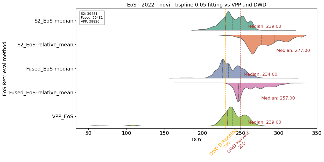

Comparing POS vs DWD and HR-VPP

# Plotting POS vs VPP reference

# Combine selected parameters from both datasets
params_to_plot1 = ['S2_max_2022_ndvi_doy']

params_to_plot2 = ['Fused_max_2022_ndvi_doy']

params_to_plot3 = ['VPP_2022_S2_T33UUT-010m_V105_s1_MAXD_utm_adjusted']

# Combine selected parameters from both datasets
df_combined = pd.concat([df_m1[params_to_plot1], df_m2[params_to_plot2], df_m3[params_to_plot3]], axis=1)

# Reshape DataFrame for Seaborn's violin plot
df_melted = pd.melt(df_combined, value_vars=params_to_plot1 + params_to_plot2 + params_to_plot3)

# Set up the plot
plt.figure(figsize=(12, 5))

# Calculate median values for each parameter
medians = df_combined.median()

# DWD fixed value for phase 65 (Tassel emergence)
#specific_value65 = 195  # Replace with the desired value
plt.axvline(x=specific_value65, color='brown', linestyle='dashed', linewidth=1, label=f'Specific Value: {specific_value65}')

# Add text to the line with vertical rotation
plt.text(specific_value65, len(params_to_plot1 + params_to_plot1 + params_to_plot3) + 0.6, f'DWD Tip of tassel\n emergence: {specific_value65}', rotation=45,
          ha='center', verticalalignment='bottom', color='brown', fontsize=10)

# Count non-NaN entries in each parameter column
s2_count = df_m1[params_to_plot1[0]].count()
fused_count = df_m2[params_to_plot2[0]].count()
vpp_count = df_m3[params_to_plot3[0]].count()

# Create the annotation text with data counts
counts_text = f"S2: {s2_count}\nFused: {fused_count}\nVPP: {vpp_count}"

# Add the text box to the plot
plt.text(0.02, 0.97, counts_text, fontsize=9, transform=plt.gca().transAxes,
         verticalalignment='top', color='black', bbox=dict(facecolor='white', alpha=0.6))

# Create a horizontal violin plot with strip plot
sns.violinplot(x='value', y='variable', data=df_melted, inner="quartile", split=True, orient='h', palette='Set2', legend=False, hue='variable')

# Display median values on the right axis with vertical offset
horizontal_offset = -20  # Adjust this value as needed
vertical_offset = 0.25  

for i, (param, median) in enumerate(medians.items()):
    plt.text(median - horizontal_offset, i + vertical_offset, f'Median: {median:.2f}', ha='left', va='center', color='brown', fontsize=12)

# Customize the plot
plt.title('PoS - 2022/ - bspline 0.05 fitting vs VPP and DWD', fontsize=14)
plt.xlabel('DOY', fontsize=14)
plt.ylabel('PoS Retrieval method', fontsize=14)
plt.tick_params(axis='both', which='major', labelsize=14)
plt.yticks(range(len(params_to_plot1 + params_to_plot2 + params_to_plot3)), ['S2_POS','Fused_POS', 'VPP_MAXD'])
plt.show()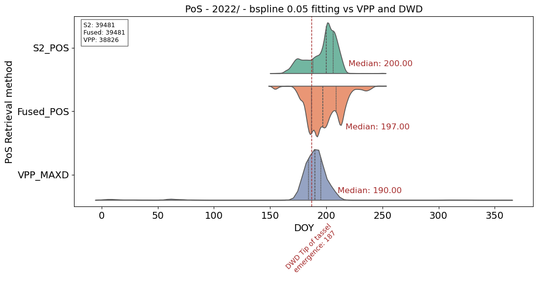

4. Error metrics calculation (RSME, MAE, Bias)

# Output folder for error files
output_directory = './Errors/'
os.makedirs(output_directory, exist_ok=True)

S2-based retrieval errors

# Calculation of error metrics for S2-based extracted phenometrics and retrieval method

# Directory with satellite-derived phenometrics
input_directory = './LSP_outputs/S2_2022_0.05_output_v1/'

# AOI shapefile
shapefile_path = './References/IACS/2022_fid13_maize_subset.shp'
aoi = gpd.read_file(shapefile_path)

# Phenometrics to evaluate
phenometrics = ['sos', 'eos', 'max']

# Reference files per phenometric
references = {
    'sos': {
        'DWD_12': r'./References/DWD/DOY_215-12_2022_resampled_10_utm_maize.tif',
        'DWD_67': r'./References/DWD/DOY_215-67_2022_resampled_10_utm_maize.tif'
    },
    'eos': {
        'DWD_20': r'./References/DWD/DOY_215-20_2022_resampled_10_utm_maize.tif',
        'DWD_24': r'./References/DWD/DOY_215-24_2022_resampled_10_utm_maize.tif'
    },
    'max': {
        'DWD_65': r'./References/DWD/DOY_215-65_2022_resampled_10_utm_maize.tif'
    }
}

def calculate_error_metrics(prediction, reference):
    mask_valid = np.isfinite(prediction) & np.isfinite(reference)
    prediction, reference = prediction[mask_valid], reference[mask_valid]
    rmse = np.sqrt(np.mean((prediction - reference) ** 2))
    mae = np.mean(np.abs(prediction - reference))
    bias = np.mean(prediction - reference)
    return rmse, mae, bias

def mask_raster_with_aoi(raster_path, aoi):
    with rasterio.open(raster_path) as src:
        out_image, out_transform = mask(src, aoi.geometry, crop=False)
        return out_image[0]

for phenometric_key in phenometrics:
    # Filter images in the directory for current phenometric
    image_paths = [
        os.path.join(input_directory, f) for f in os.listdir(input_directory)
        if f.endswith('.tif') and f"_{phenometric_key}_" in f.lower()
    ]

    if not image_paths:
        print(f"No files found for {phenometric_key}")
        continue

    for ref_name, reference_path in references[phenometric_key].items():
        print(f"\nProcessing: {phenometric_key.upper()} with reference: {ref_name}")

        # Load and mask the reference inside the loop
        try:
            ref_data = mask_raster_with_aoi(reference_path, aoi)
        except FileNotFoundError:
            print(f"Reference file not found: {reference_path}")
            continue

        # Initialize metric lists
        methods = []
        rmse_values = []
        mae_values = []
        bias_values = []

        # Loop through each method image
        for image_path in image_paths:
            method_name = os.path.basename(image_path).split(".")[0]
            methods.append(method_name)

            try:
                prediction_data = mask_raster_with_aoi(image_path, aoi)
                rmse, mae, bias = calculate_error_metrics(prediction_data, ref_data)
            except Exception as e:
                print(f"Error processing {image_path}: {e}")
                rmse, mae, bias = np.nan, np.nan, np.nan

            rmse_values.append(rmse)
            mae_values.append(mae)
            bias_values.append(bias)

        # Compile metrics
        df_metrics = pd.DataFrame({
            'Method': methods,
            'RMSE': rmse_values,
            'MAE': mae_values,
            'Bias': bias_values
        })

        df_metrics = df_metrics.sort_values(by='MAE')

        # Save CSV
        output_csv = os.path.join(
            output_directory, f"S2_{phenometric_key.upper()}_error_metrics_{ref_name}.csv"
        )
        df_metrics.to_csv(output_csv, index=False)
        print(f"Saved results to: {output_csv}")

        print(f"\n=== Error metrics for {phenometric_key.upper()} using reference {ref_name} ===")
        print(df_metrics.round(3).to_string(index=False))
        print("-" * 50)

Fused-based retrieval errors

# Calculation of error metrics for Fused-based extracted phenometric and retrieval method

# Directory with satellite-derived phenometrics
input_directory = './LSP_outputs/Fused_2022_0.05_output_v1/'

# AOI shapefile
shapefile_path = './References/IACS/2022_fid13_maize_subset.shp'
aoi = gpd.read_file(shapefile_path)

# Phenometrics to evaluate
phenometrics = ['sos', 'eos', 'max']

# Reference files per phenometric
references = {
    'sos': {
        'DWD_12': r'./References/DWD/DOY_215-12_2022_resampled_10_utm_maize.tif',
        'DWD_67': r'./References/DWD/DOY_215-67_2022_resampled_10_utm_maize.tif'
    },
    'eos': {
        'DWD_20': r'./References/DWD/DOY_215-20_2022_resampled_10_utm_maize.tif',
        'DWD_24': r'./References/DWD/DOY_215-24_2022_resampled_10_utm_maize.tif'
    },
    'max': {
        'DWD_65': r'./References/DWD/DOY_215-65_2022_resampled_10_utm_maize.tif'
    }
}

def calculate_error_metrics(prediction, reference):
    mask_valid = np.isfinite(prediction) & np.isfinite(reference)
    prediction, reference = prediction[mask_valid], reference[mask_valid]
    rmse = np.sqrt(np.mean((prediction - reference) ** 2))
    mae = np.mean(np.abs(prediction - reference))
    bias = np.mean(prediction - reference)
    return rmse, mae, bias

def mask_raster_with_aoi(raster_path, aoi):
    with rasterio.open(raster_path) as src:
        out_image, out_transform = mask(src, aoi.geometry, crop=False)
        return out_image[0]  # First band

for phenometric_key in phenometrics:
    # Filter images in the directory for current phenometric
    image_paths = [
        os.path.join(input_directory, f) for f in os.listdir(input_directory)
        if f.endswith('.tif') and f"_{phenometric_key}_" in f.lower()
    ]

    if not image_paths:
        print(f"No files found for {phenometric_key}")
        continue

    for ref_name, reference_path in references[phenometric_key].items():
        print(f"\nProcessing: {phenometric_key.upper()} with reference: {ref_name}")

        # Load and mask the reference inside the loop
        try:
            ref_data = mask_raster_with_aoi(reference_path, aoi)
        except FileNotFoundError:
            print(f"Reference file not found: {reference_path}")
            continue

        # Initialize metric lists
        methods = []
        rmse_values = []
        mae_values = []
        bias_values = []

        # Loop through each method image
        for image_path in image_paths:
            method_name = os.path.basename(image_path).split(".")[0]
            methods.append(method_name)

            try:
                prediction_data = mask_raster_with_aoi(image_path, aoi)
                rmse, mae, bias = calculate_error_metrics(prediction_data, ref_data)
            except Exception as e:
                print(f"Error processing {image_path}: {e}")
                rmse, mae, bias = np.nan, np.nan, np.nan

            rmse_values.append(rmse)
            mae_values.append(mae)
            bias_values.append(bias)

        # Compile metrics
        df_metrics = pd.DataFrame({
            'Method': methods,
            'RMSE': rmse_values,
            'MAE': mae_values,
            'Bias': bias_values
        })

        df_metrics = df_metrics.sort_values(by='MAE')

        # Save CSV
        output_csv = os.path.join(
            output_directory, f"Fused_{phenometric_key.upper()}_error_metrics_{ref_name}.csv"
        )
        df_metrics.to_csv(output_csv, index=False)
        print(f"Saved results to: {output_csv}")

        print(f"\n=== Error metrics for {phenometric_key.upper()} using reference {ref_name} ===")
        print(df_metrics.round(3).to_string(index=False))
        print("-" * 50)

5. Error metrics differences per phenometric

# Calculating error metrics differences 

output_directory = r'./Errors/'

diffs = []

# Get all S2 files
s2_files = [f for f in os.listdir(output_directory) if f.startswith("S2_") and f.endswith(".csv")]

for s2_file in s2_files:
    fused_file = s2_file.replace("S2_", "Fused_")
    s2_path = os.path.join(output_directory, s2_file)
    fused_path = os.path.join(output_directory, fused_file)

    if not os.path.exists(fused_path):
        print(f"Skipping {s2_file}, fused file not found.")
        continue

    s2_df = pd.read_csv(s2_path)
    fused_df = pd.read_csv(fused_path)

    # --- Extract method name from column like 'S2_sos_relative_amplitude_' ---
    def extract_method(full_string):
        parts = full_string.strip('_').split('_')
        return parts[3] if len(parts) > 2 else full_string

    s2_df['Method_clean'] = s2_df['Method'].apply(extract_method)
    fused_df['Method_clean'] = fused_df['Method'].apply(extract_method)

    # Merge on cleaned method name
    merged = pd.merge(
        s2_df, fused_df,
        on='Method_clean',
        suffixes=('_S2', '_Fused')
    )

    if merged.empty:
        print(f"No matched methods in: {s2_file}")
        continue

    # Get ref and phenometric from filename
    parts = s2_file.split('_')
    phenometric = parts[1]
    ref = parts[-1].replace('.csv', '')

    # Calculate differences (Fused - S2)
    merged['RMSE_diff'] = merged['RMSE_Fused'] - merged['RMSE_S2']
    merged['MAE_diff'] = merged['MAE_Fused'] - merged['MAE_S2']
    merged['Bias_diff'] = merged['Bias_Fused'] - merged['Bias_S2']

    merged['Ref'] = ref
    merged['Phenometric'] = phenometric
    merged['Method'] = merged['Method_clean']

    diffs.append(merged[['Method', 'Ref', 'Phenometric', 'RMSE_diff', 'MAE_diff', 'Bias_diff']])

# Combine all
df_diffs = pd.concat(diffs, ignore_index=True)
df_diffs.to_csv(os.path.join(output_directory, 'Combined_differences.csv'), index=False)

print("\n DONE: Combined difference:")
print(df_diffs)

6. Box plot comparison on error metrics - Fused vs S2 improvement

input_file = './Errors/Combined_differences.csv'
df = pd.read_csv(input_file)

# Define reference code related to phenological stage

ref_labels = {
    12: "Emergence",
    67: "Shooting",
    65: "Tassel Emergence",
    20: "Dough Ripening",
    24: "Harvest"
}

df["Ref_Label"] = df["Ref"].map(ref_labels)

# Melting data
df_melted = df.melt(
    id_vars=["Method", "Ref", "Ref_Label", "Phenometric"],
    value_vars=["RMSE_diff", "MAE_diff", "Bias_diff"],
    var_name="Metric",
    value_name="Diff"
)

base_palette = sns.color_palette("Set2")
unique_methods = df["Method"].unique()

custom_colors = {
    'Median': 'blue',
    'Relative': 'red'
}

method_palette = {
    method: custom_colors.get(method, base_palette[i % len(base_palette)])
    for i, method in enumerate(unique_methods)
}

# Plotting box plots per phenometrics and method
sns.set(style="whitegrid")
phenometrics = ['SOS', 'MAX', 'EOS']

for phen in phenometrics:
    sub = df_melted[df_melted['Phenometric'] == phen]

    g = sns.catplot(
        data=sub,
        kind='bar',
        x='Ref_Label',
        y='Diff',
        hue='Method',
        col='Metric',
        col_order=["RMSE_diff", "MAE_diff", "Bias_diff"],
        palette=method_palette,
        height=5,
        aspect=0.8
    )

    # Set consistent y-axis range
    g.set(ylim=(-25, 25))
    g.fig.subplots_adjust(top=0.8)
    g.fig.suptitle(f"{phen}", fontsize=16)

    for ax in g.axes.flat:
        # Shaded zones
        ax.axhspan(-25, 0, facecolor='green', alpha=0.1)
        ax.axhspan(0, 25, facecolor='red', alpha=0.1)

        # Horizontal zero line
        ax.axhline(0, color='black', linestyle='--', linewidth=1)

        # Right-side secondary y-axis with vertical labels
        secax = ax.secondary_yaxis('right', functions=(lambda y: y, lambda y: y))
        secax.set_ylim(ax.get_ylim())
        secax.set_yticks([-10, -5, 18, 20])  # Adjust tick positions for upper emphasis
        secax.set_yticklabels(['Fused better', '', 'S2 better', ''])
        secax.tick_params(axis='y', colors='gray', labelrotation=90, pad=10)

        ax.set_xlabel('')
        ax.set_ylabel('Difference (Fused - S2)')

    plt.show()