Section 3

Geospatial data handling; groundwater time series and covariates

Estimated Time: ~30 minutes

Covariates were chosen based on their established impact on the groundwater table head fluctuations (Amanambu et al., 2020; Condon and Maxwell, 2015; Glanville et al., 2023). See section 1 for details

Load required libraries

library(raster)
library(sp)
library(rgdal)
library(dplyr)
library(ggplot2)
library(meteo)
library(rstudioapi)

Define base path and working directory

base_path <- "C:/Users/raza/project"
set.seed(42)
RNGkind(kind = "Mersenne-Twister", normal.kind = "Inversion", sample.kind = "Rejection")

wd <- dirname(rstudioapi::getActiveDocumentContext()$path)
setwd(wd)

Load boundary shapefile and define coordinate systems

utm33 <- "+proj=utm +zone=32 +ellps=WGS84 +datum=WGS84 +units=m +no_defs"
border_wgs84 <- readOGR(paste0(base_path, "/borders/Brandenburg1.shp"))
border <- spTransform(border_wgs84, CRS(utm33))

Create directory for plots if not present

if (!dir.exists("plot")) dir.create("plot")

Define variables

v <- "GWD"
year <- "2001-05"
covariates <- c("GWD", "Lat", "Lon", "SLOPE", "ASP", "DEM", 
                "LNF", "TPI", "TWI", "TRI", "PREC", "TEMP", 
                "NDVI", "ET", "EVI")

Convert cleaned CSV data to space-time object (STFDF)

for (year in "2001-05") {

  # Load cleaned dataset
  file_name <- paste0(base_path, "/clean_", year, ".csv")
  bran <- read.csv(file_name)[, -1]
  bran <- na.omit(bran)

  # Format date
  bran$DATE <- as.Date(paste0(bran$DATE, "-01"), format = "%b-%y-%d")

  # Extract observation and station information
  ob <- bran[, c(5, 6, 10, 18, 19, 20, 21, 22)]
  sta <- bran[, c(5, 3, 4, 7, 8, 11, 12, 13, 14, 15, 16, 17)]
  sta <- sta[!duplicated(sta), ]

  # Create space-time data structure
  stfdf <- meteo2STFDF(
    obs = ob,
    stations = sta,
    crs = CRS(utm33),
    obs.staid.time = c(1, 2),
    stations.staid.lon.lat = c(1, 4, 5)
  )

  stfdf@sp@data$staid <- 1:nrow(stfdf@sp)

  # Save STFDF object for future use
  # save(stfdf, file = paste0("stfdf_", year, ".rda"))
}

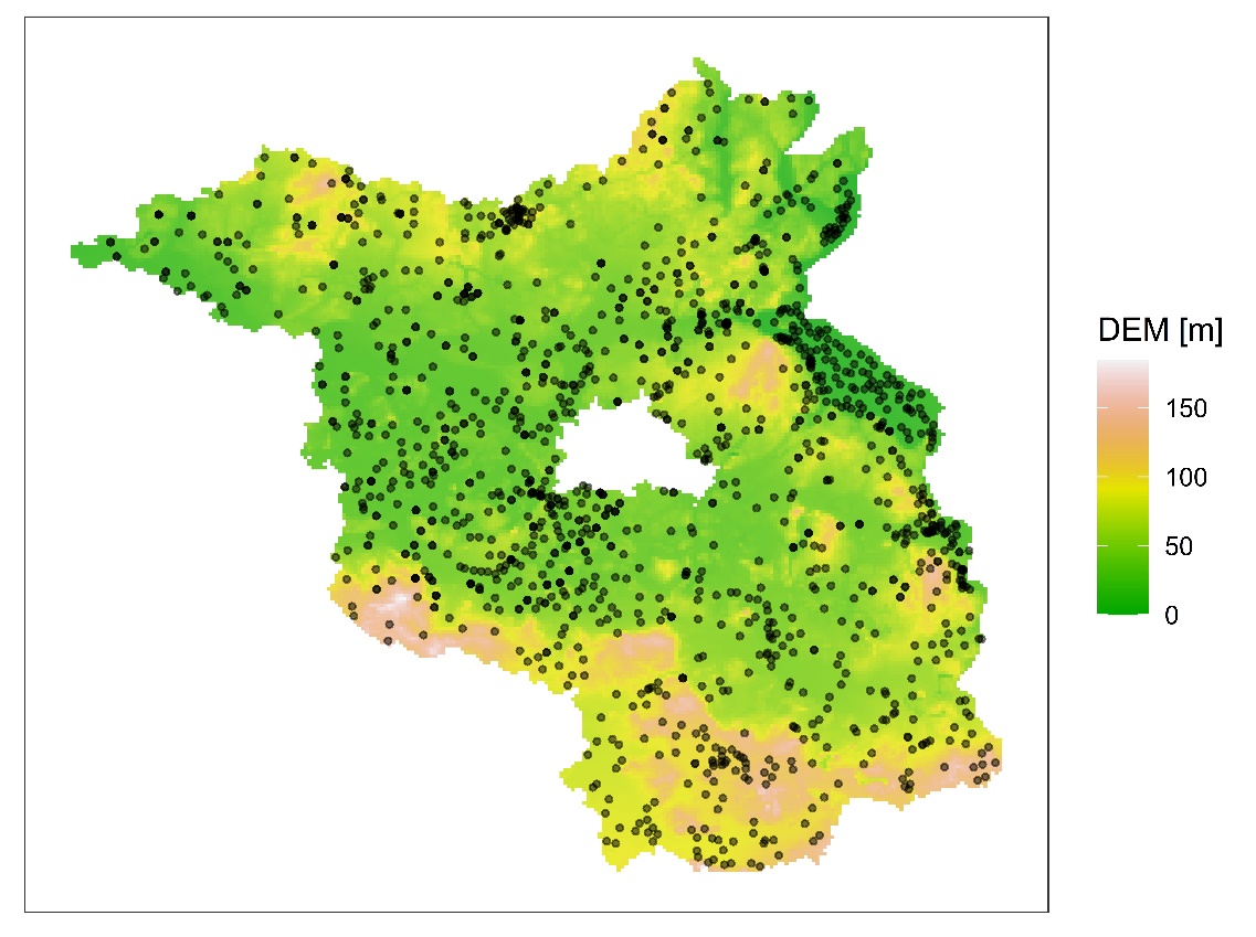
VISUALIZATION 1: STATION LOCATIONS OVER DEM

# Load processed STFDF data
load("stfdf_2001-05.rda")

# Convert spatial projection
stfdf@sp <- spTransform(stfdf@sp, CRS("+proj=utm +zone=31 +ellps=WGS84 +datum=WGS84 +units=m +no_defs"))

# Load and project DEM raster
r <- raster("DEM.tif")
r <- projectRaster(r, crs = CRS("+proj=utm +zone=32 +ellps=WGS84 +datum=WGS84 +units=m +no_defs"))
r <- as(r, "SpatialPixelsDataFrame")

# Create base map with station points
sta_dem_plot <- ggplot() +
  geom_raster(data = as.data.frame(r), aes(x = x, y = y, fill = DEM), alpha = 0.8) +
  geom_point(data = as.data.frame(stfdf@sp), aes(x = lon, y = lat), size = 0.8, alpha = 0.5) +
  scale_fill_gradientn(colours = terrain.colors(100), name = "DEM [m]") +
  labs(x = "Longitude", y = "Latitude") +
  theme_bw() +
  theme(
    legend.position = "right",
    plot.title = element_text(hjust = 0.5, face = "bold"),
    axis.title = element_blank(),
    axis.ticks = element_blank(),
    axis.text.x = element_blank(),
    axis.text.y = element_blank(),
    panel.grid = element_blank()
  )

# Export figure
jpeg("../plot/stations.jpeg", width = 150, height = 112, units = 'mm', res = 1800)
print(sta_dem_plot)
dev.off()

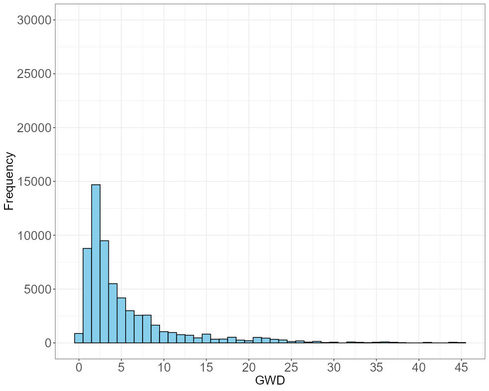
VISUALIZATION 2: HISTOGRAM OF GROUNDWATER DEPTH (GWD)

his <- ggplot(stfdf@data, aes(x = GWD)) +
  geom_histogram(binwidth = 1, fill = "skyblue", color = "black") +
  labs(x = "GWD", y = "Frequency") +
  scale_x_continuous(breaks = seq(0, max(stfdf@data$GWD, na.rm = TRUE), by = 5)) +
  scale_y_continuous(limits = c(0, 30000), breaks = seq(0, 30000, by = 5000)) +
  theme_bw() +
  theme(
    plot.title = element_text(size = 18, face = "bold"),
    axis.title = element_text(size = 18),
    axis.text = element_text(size = 18)
  )

# Save histogram
ggsave(filename = "../plot/histogram.jpeg", plot = his, width = 25, height = 20, units = "cm", dpi = 100)