Section 6
Conventional ML – RFSI
Estimated Time: ~25 minutes
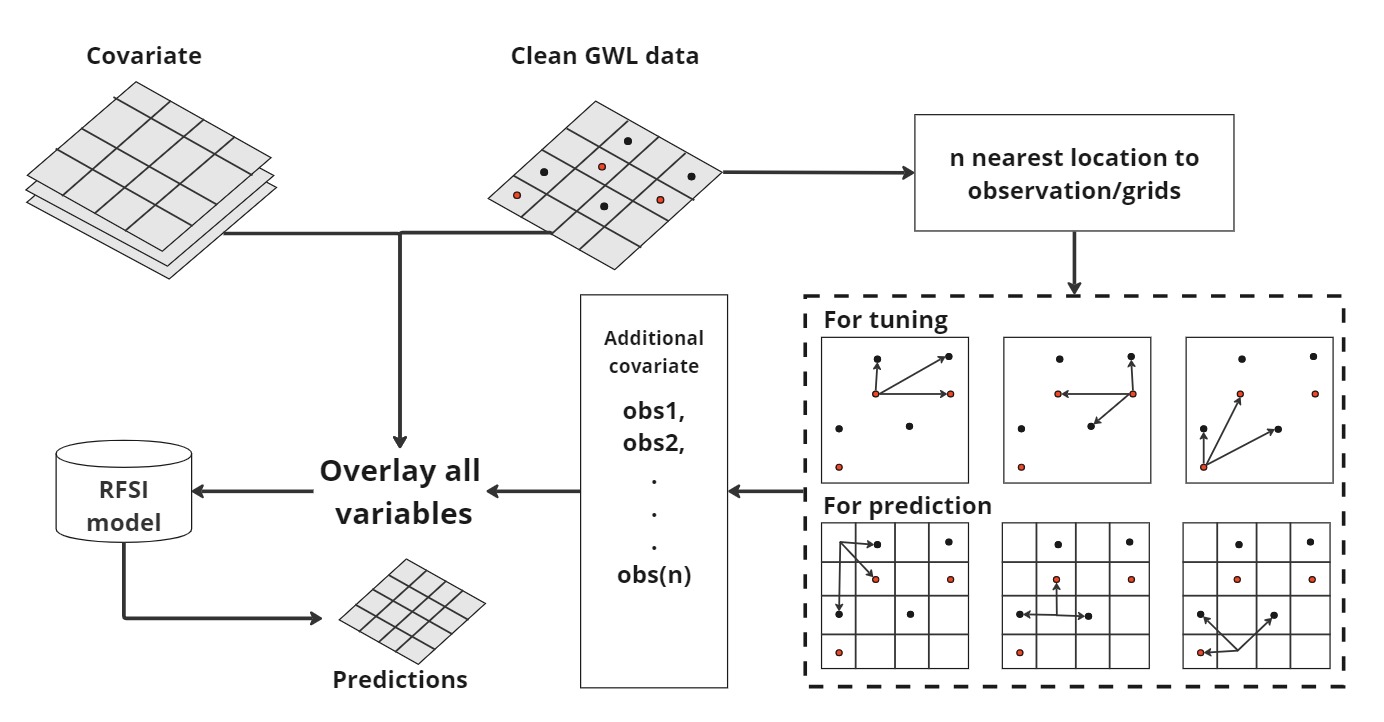
In this section, we apply the Random Forest Spatial Interpolation (RFSI) method to improve groundwater level predictions. Standard Random Forest models do not explicitly account for spatial autocorrelation, except indirectly through spatially correlated covariates. Since nearby observations provide valuable information for estimating values at unsampled locations, we enhance the model by including additional spatial covariates. These covariates represent the observed values at the n nearest locations and the corresponding distances between these locations and each prediction point (Fig. 1)
Inputs:
- Grid based MODIS ET, NDVI, EVI values
- Temperature and precipitation data from German weather station (DWD)
- Coordinates
- observations at n nearest locations
- distance of each observation from these locations
Output
- Trained RFsp model
- Write trained model predictions on the testing data set.
- Tuned set of model parameters
- Computational time
Section 6
Conventional ML – RFSI

####################################
setwd("C:/Users/raza/project")
base_path <- "C:/Users/raza/project/plot"
year_ranges <- c("2001-05")

# Loop through years from 2001 to 2005
for (year in year_ranges) {
  start_time <- Sys.time()
  cat("Processing year:", year, "\n")
  file_name <- paste0("stfdf_", year, ".rda")

  # Load spatiotemporal data frame for the current year
  load(file = file_name)

  # Convert the data to a format suitable for modeling
  GWD_df <- as.data.frame(stfdf)

  covariates <- c("GWD", "Lat", "Lon", "SLOPE", "ASP", "DEM", "LNF", "TPI", "TWI", "TRI", "PREC", "TEMP", "NDVI", "ET", "EVI")
  GWD_df <- GWD_df[, c("Lon", "Lat", "sp.ID", "time", covariates)]
  GWD_df = GWD_df[complete.cases(GWD_df), ]

  time = sort(unique(GWD_df$time))
  daysNum = length(time)
  days = gsub("-", "", time, fixed=TRUE)

  nos <- 6:14
  min.node.size <- 5:6
  #min.node.size <- 4:6 # 2:6
  sample.fraction <- seq(1, 0.632, -0.05)
  ntree <- 250

  n_obs = max(nos)
  #mtry <- 3:(9 + 2 * n_obs)
  mtry <- 3

  indices <- CreateSpacetimeFolds(GWD_df, spacevar = "sp.ID", k = 5, seed = 42)

  hp <- expand.grid(min.node.size = min.node.size, mtry = mtry, no = nos, sf = sample.fraction)
  hp <- hp[hp$mtry < (9 + 2 * hp$no - 1), ]
  hp <- hp[sample(nrow(hp), 100), ]
  hp <- hp[order(hp$no), ]
  rmse_hp <- rep(NA, nrow(hp))

  lowest_rmse <- Inf  # Initialize with a high value
  iteration_since_lowest <- 0  # Counter for iterations since the lowest RMSE

  for (h in 1:nrow(hp)) {
    comb <- hp[h, ]
    print(paste("combination: ", h, sep = ""))
    print(comb)

    dev_df <- GWD_df

    fold_obs <- c()
    fold_pred <- c()

    for (f in 1:length(indices$index)) {
      print(paste("fold: ", f, sep = ""))
      cols <- c(covariates, paste("dist", 1:(comb$no), sep = ""), paste("obs", 1:(comb$no), sep = ""))
      dev_df1 <- dev_df[indices$index[[f]], ]

      cpus <- detectCores() - 1
      registerDoParallel(cores = cpus)
      nearest_obs <- foreach (t = time) %dopar% {
        dev_day_df <- dev_df1[as.numeric(dev_df1$time) == t, c("Lon", "Lat", "GWD")]
        day_df <- dev_df[as.numeric(dev_df$time) == as.numeric(t), c("Lon", "Lat", "GWD")]

        if (nrow(day_df) == 0) {
          return(NULL)
        }
        return(meteo::near.obs(
          locations = day_df,
          observations = dev_day_df,
          obs.col = "GWD",
          n.obs = comb$no
        ))
      }

      stopImplicitCluster()

      nearest_obs <- do.call("rbind", nearest_obs)
      dev_df <- cbind(dev_df, nearest_obs)
      dev_df = dev_df[complete.cases(dev_df), ]

      dev_df1 <- dev_df[indices$index[[f]], cols]
      dev_df1 <- dev_df1[complete.cases(dev_df1), ]
      val_df1 <- dev_df[indices$indexOut[[f]], cols]
      val_df1 <- val_df1[complete.cases(val_df1), ]

      model <- ranger(GWD ~ ., data = dev_df1, importance = "none", seed = 42,
                      num.trees = ntree, mtry = comb$mtry,
                      splitrule = "variance",  # variance extratrees
                      min.node.size = comb$min.node.size,
                      sample.fraction = comb$sf,
                      oob.error = FALSE)
      fold_obs <- c(fold_obs, val_df1$GWD)
      fold_pred <- c(fold_pred, predict(model, val_df1)$predictions)
    }

    rmse_hp[h] <- sqrt(mean((fold_obs - fold_pred)^2, na.rm = TRUE))
    print(paste("rmse: ", rmse_hp[h], sep = ""))

    if (rmse_hp[h] < lowest_rmse) {
      lowest_rmse <- rmse_hp[h]
      iteration_since_lowest <- 0  # Reset counter
      print(paste("New lowest RMSE:", lowest_rmse))
    } else {
      iteration_since_lowest <- iteration_since_lowest + 1
      print(paste("Iterations since lowest RMSE:", iteration_since_lowest))
    }

    # Stop if 5 iterations have passed since the lowest RMSE was found
    if (iteration_since_lowest >= 5) {
      print(paste("Stopping after", iteration_since_lowest, "iterations since the lowest RMSE"))
      break
    }
  }

  dev_parameters <- hp[which.min(rmse_hp), ]
  print(dev_parameters)

  cpus <- detectCores() - 1
  registerDoParallel(cores = cpus)

  nearest_obs <- foreach (t = time) %dopar% {
    day_df <- GWD_df[GWD_df$time == t, c("Lon", "Lat", "GWD")]
    if (nrow(day_df) == 0) {
      return(NULL)
    }
    return(near.obs(
      locations = day_df,
      observations = day_df,
      obs.col = "GWD",
      n.obs = dev_parameters$no
    ))
  }

  stopImplicitCluster()

  nearest_obs <- do.call("rbind", nearest_obs)
  GWD_df <- cbind(GWD_df, nearest_obs)

  cols <- c(covariates, paste("dist", 1:(dev_parameters$no), sep = ""), paste("obs", 1:(dev_parameters$no), sep = ""))
  GWD_df <- GWD_df[, cols]
  colnames(GWD_df)
  a <- GWD_df
  # Identify unique combinations of latitude and longitude
  unique_coords <- unique(GWD_df[, c("Lat", "Lon")])

  # Set a seed for reproducibility
  set.seed(123)

  # Create an index for splitting the data
  index <- createDataPartition(1:nrow(unique_coords), p = 0.8, list = FALSE)

  # Use the index to split the unique coordinates into training and testing sets
  train_coords <- unique_coords[index, ]
  test_coords <- unique_coords[-index, ]

  # Merge the original data with the training and testing coordinates
  train_data <- merge(GWD_df, train_coords, by = c("Lat", "Lon"))
  test_data <- merge(GWD_df, test_coords, by = c("Lat", "Lon"))
  nrow(test_data)
  write_csv(test_data, "test_data_lat_lon.csv")
  # Select covariates
  covariates <- colnames(GWD_df)
  covariates <- covariates[covariates != "GWD"]  # Assuming "GWD" is the response variable

  # Subset the data frames with selected covariates
  train_data <- train_data[, c("GWD", covariates)]
  test_data <- test_data[, c("GWD", covariates)]

  rfsi_model <- ranger(GWD ~ ., data = train_data, importance = "impurity", seed = 42,
                       num.trees = ntree, mtry = dev_parameters$mtry,
                       splitrule = "extratrees",
                       min.node.size = dev_parameters$min.node.size,
                       sample.fraction = dev_parameters$sf,
                       quantreg = TRUE)  ### quantreg???

  # save(rfsi_model, file = "../models/RFSI.rda")
  save(rfsi_model, file = paste0("../models/RFSI_", year, ".rda"))

  # Create and save plot_data
  plot_data <- data.frame(Lat = train_data$Lat, Lon = train_data$Lon, Observations = train_data$GWD, Predictions = rfsi_model$predictions)
  plot_file <-  paste0(base_path, (paste0("\\model_training\\rfsi_training_", year, ".csv")))
  write.csv(plot_data, plot_file)

  # Make predictions on the test data using the trained model
  predictions <- predict(rfsi_model, data = test_data, type = "response")

  # Add the predictions to the test_data dataframe
  test_data$predicted_GWD <- predictions$predictions

  #test_data <- test_data[, c("GWD", "predicted_GWD")]

  plot_data_test <- data.frame(Lat = test_data$Lat, Lon = test_data$Lon, GWD = test_data$GWD, predicted_GWD = test_data$predicted_GWD)
  # Save test_data with predictions as a CSV file
  test_file <-  paste0(base_path, (paste0("\\model_testing\\rfsi_test_", year, ".csv")))
  write.csv(plot_data_test, test_file)

  end_time <- Sys.time()
  computation_time <- end_time - start_time
  #cat("dev_parameters for year", year, ":", dev_parameters, "\n")
  cat("Computation time for year", year, ":", computation_time, "\n")

  # Save dev_parameters, RMSE, and computation_time to a text file
  result_file <- paste0(base_path, "\\computation_times_rfsi.txt")
  write(paste("Year:", year), file = result_file, append = TRUE)
  write(paste("dev_parameters:", toString(dev_parameters)), file = result_file, append = TRUE)
  write(paste("RMSE:", min(rmse_hp, na.rm = TRUE)), file = result_file, append = TRUE)
  write(paste("Computation time:", computation_time), file = result_file, append = TRUE)
  write("\n", file = result_file, append = TRUE)
}