Section 8

Time Series Mapping of Groundwater Levels

Estimated Time: ~30 minutes

Now let’s use the trained models to generate groundwater-level predictions across the study area. Raster datasets will be imported to visualize spatial patterns in the predicted groundwater dynamics. Time-indexed rasters will enable temporal analyses and animations to track changes across seasons and years. All layers will be harmonized in projection, resolution, and extent to ensure accurate spatiotemporal comparisons.

Define target year, file paths, and shapefile

base_path <- "C:/Users/raza"
target_year <- "2002"

folder_paths <- c(
  "C:/Users/raza/project/ET",
  "C:/Users/raza/project/EVI",
  "C:/Users/raza/project/NDVI",
  "C:/Users/raza/project/Prec",
  "C:/Users/raza/project/Temp"
)

# Load reference raster for projection and alignment
reference_raster <- raster("C:/Users/raza/project/ASP.tif")
reference_coordinates <- coordinates(reference_raster)

# Load and reproject shapefile
shapefile <- readOGR("C:/Users/raza/project/borders/Brandenburg.shp")
shapefile <- spTransform(shapefile, CRS("+proj=utm +zone=32 +datum=WGS84 +units=m +no_defs"))

# Initialize empty dataframe for results
final_data <- data.frame(Date = as.Date(character(0)), Value = numeric(0), X = numeric(0), Y = numeric(0))

Loop through raster folders and extract values

extract_layer_data <- function(folder_path, target_year, reference_raster, shapefile) {
  folder_data <- data.frame()

  files <- list.files(folder_path, pattern = "\\.tif$", full.names = TRUE)

  for (month in 1:12) {
    matching_files <- grep(paste0(target_year, ".", sprintf("%02d", month)), files, value = TRUE)

    for (file_path in matching_files) {
      raster_layer <- raster(file_path)
      raster_layer <- projectRaster(raster_layer, crs = crs(reference_raster))
      raster_layer <- crop(raster_layer, extent(shapefile))
      raster_layer <- mask(raster_layer, shapefile)

      values <- extract(raster_layer, reference_coordinates)
      coords <- coordinates(reference_raster)

      date <- as.Date(paste(target_year, sprintf("%02d", month), "01", sep = "-"))
      variable_name <- substr(basename(file_path), 1, 3)

      new_row <- data.frame(Date = date, Value = values, X = coords[,1], Y = coords[,2])
      colnames(new_row)[colnames(new_row) == "Value"] <- variable_name

      folder_data <- bind_rows(folder_data, new_row)
    }
  }
  return(folder_data)
}

# Loop through all folders and combine
for (folder in folder_paths) {
  folder_data <- extract_layer_data(folder, target_year, reference_raster, shapefile)
  final_data <- bind_rows(final_data, folder_data)
}

Reshape and clean data

# Pivot to wide format based on raster variable names
final_data_wide <- final_data %>%
  group_by(Date, X, Y) %>%
  summarise_all(list(~ if(all(is.na(.))) NA else na.omit(.))) %>%
  ungroup()

final_data_wide <- na.omit(final_data_wide)

# Save wide data for predictions
write.csv(final_data_wide, "C:/Users/raza/project/data_for_pred_2022.csv", row.names = FALSE)

Extract raster values for additional layers

raster_dir <- "C:/Users/raza/project/brandenburg"
raster_files <- list.files(raster_dir, pattern = "\\.tif$", full.names = TRUE)
csv_data <- read.csv("C:/Users/raza/project/data_for_pred_2022.csv")

extract_raster_values <- function(raster_file, x, y) {
  raster_layer <- raster(raster_file)
  extract(raster_layer, cbind(x, y))
}

for (raster_file in raster_files) {
  raster_name <- sub(".tif", "", basename(raster_file))
  csv_data[[raster_name]] <- extract_raster_values(raster_file, csv_data$X, csv_data$Y)
}

# Reorder and scale columns
desired_order <- c("Date", "X", "Y", "SLOPE", "ASP", "DEM", "LNF", "TPI", "TWI", "TRI", "PREC", "TEMP", "NDVI", "ET", "EVI")
csv_data <- csv_data[, desired_order]
csv_data$NDVI <- csv_data$NDVI / 10000

# Convert coordinates to WGS84
coordinates(csv_data) <- ~ X + Y
proj4string(csv_data) <- CRS("+proj=utm +zone=32 +datum=WGS84 +units=m +no_defs")
csv_data <- spTransform(csv_data, CRS("+proj=longlat +datum=WGS84"))

csv_data$Lon <- coordinates(csv_data)[,1]
csv_data$Lat <- coordinates(csv_data)[,2]

# Save final CSV
write.csv(csv_data, "C:/Users/raza/project/b_data_for_prediction/data_for_pred_2022_v2.csv", row.names = FALSE)

Create Monthly Prediction Rasters using Random Forest Model

library(raster)
library(sp)
library(dplyr)

# -----------------------------
# Define directories and paths
# -----------------------------
model_dir <- file.path(base_path, "project/models")
test_data_dir <- file.path(base_path, "project", "b_data_for_prediction")
output_dir <- file.path(base_path, "project/plot")
reference_raster_path <- file.path(base_path, "project/brandenburg", "DEM.tif")

# -----------------------------
# Prepare reference raster
# -----------------------------
reference_raster <- raster(reference_raster_path)
projected_raster <- projectRaster(reference_raster, crs = CRS("+proj=longlat +datum=WGS84"))
template_raster <- raster(projected_raster)

# -----------------------------
# Load trained Random Forest model
# -----------------------------
model_file <- file.path(model_dir, "RF_2001-05.rda")
load(model_file)

# -----------------------------
# Process data year by year
# -----------------------------
for (year in 2001:2005) {

  test_data_file <- file.path(test_data_dir, paste0("data_for_pred_", year, "_v2.csv"))
  if (!file.exists(test_data_file)) {
    message(paste("File not found:", test_data_file))
    next
  }

  test_data <- read.csv(test_data_file) %>% na.omit()

  if (nrow(test_data) == 0) {
    message(paste("No valid data for year:", year))
    next
  }

  # Predict groundwater or variable of interest
  preds <- predict(rf_model, data = test_data)
  test_data$Predictions <- preds$predictions

  # Ensure Date is in proper format
  test_data$Date <- as.Date(test_data$Date)
  unique_months <- sort(unique(format(test_data$Date, "%Y-%m")))

  # -----------------------------
  # Create monthly rasters
  # -----------------------------
  for (month in unique_months) {

    month_data <- test_data %>%
      filter(format(Date, "%Y-%m") == month)

    if (nrow(month_data) == 0) next

    # Convert to spatial points
    sp_data <- month_data %>%
      select(Lon, Lat, Predictions)
    coordinates(sp_data) <- c("Lon", "Lat")

    # Rasterize
    monthly_raster <- rasterize(sp_data, template_raster, field = "Predictions", fun = mean)

    # Define output path
    output_file <- file.path(output_dir, paste0("monthly_rf_", month, ".tif"))

    # Write raster
    writeRaster(monthly_raster, filename = output_file, format = "GTiff", overwrite = TRUE)
  }

  message(paste("Completed processing for year:", year))
}

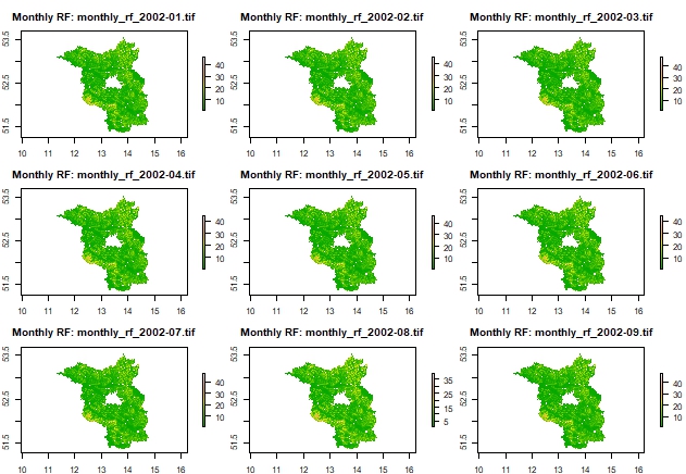
Plot 3x3 grid of monthly rasters as examples

# Get list of created rasters
raster_files <- list.files(output_dir, pattern = "monthly_rf_.*\\.tif$", full.names = TRUE)

# Check and plot up to 9 rasters
if (length(raster_files) > 0) {
  num_to_plot <- min(9, length(raster_files))
  selected_files <- raster_files[1:num_to_plot]

  # Set plotting layout
  par(mfrow = c(3, 3), mar = c(2, 2, 3, 4))

  for (i in seq_along(selected_files)) {
    r <- raster(selected_files[i])
    plot(r, main = paste0("Monthly RF: ", basename(selected_files[i])),
         col = terrain.colors(100))
  }

  par(mfrow = c(1, 1))  # Reset layout
} else {
  message("No raster files found for plotting.")
}

Create monthly rasters using RFsp model

# Load libraries
library(doParallel)
library(landmap)
library(raster)
library(data.table)
library(dplyr)
library(plyr)

# Define directories
model_dir <- file.path(base_path, "project/models")
test_data_dir <- file.path(base_path, "project", "b_data_for_prediction")
output_dir <- file.path(base_path, "project/plot")
reference_raster_path <- file.path(base_path, "project/brandenburg", "DEM.tif")

# Load RFsp model
model_file <- file.path(model_dir, "RFsp_2001-05.rda")
load(model_file)

# Load reference raster and project to WGS84
reference_raster <- raster(reference_raster_path)
new_crs <- CRS("+proj=longlat +datum=WGS84")
reference_raster <- projectRaster(reference_raster, crs = new_crs)

# Function to create monthly rasters for a given year
process_year <- function(year) {

  message("Processing year: ", year)

  # Load test data
  test_data_file <- file.path(test_data_dir, paste0("data_for_pred_1", year, "_v2.csv"))
  if (!file.exists(test_data_file)) {
    warning("File not found: ", test_data_file)
    return(NULL)
  }

  test_data <- fread(test_data_file) %>% na.omit()
  test_data[, staid := .I]

  # Define bounding box and create fishnet grid
  bbox <- extent(min(test_data$Lon), max(test_data$Lon), min(test_data$Lat), max(test_data$Lat))
  bbox <- as(bbox, "SpatialPolygons")
  proj4string(bbox) <- new_crs

  fishnet <- raster(bbox)
  res(fishnet) <- c(0.01, 0.01)
  fishnet[] <- runif(ncell(fishnet))
  fishnet <- as(fishnet, "SpatialPixelsDataFrame")

  # Prepare date list
  unique_dates <- unique(test_data$Date)
  final_results <- list()

  for (date in unique_dates) {
    message("  Processing date: ", date)

    # Filter and prepare spatial data
    date_data <- test_data[Date == date]
    spatial_points <- SpatialPointsDataFrame(coords = date_data[, .(Lon, Lat)], data = date_data, proj4string = new_crs)

    # Compute buffer distances
    dist_map <- landmap::buffer.dist(spatial_points["staid"], fishnet[1], as.factor(1:nrow(spatial_points)))

    # Join distance info with test data
    merged_data <- cbind(date_data, over(spatial_points, dist_map))
    merged_data <- plyr::join(date_data, merged_data, by = "staid")

    # Select and reorder columns
    vars <- c("Date", "Lat", "Lon", "SLOPE", "ASP", "DEM", "LNF", "TPI", "TWI", "TRI", "PREC", "TEMP", "NDVI", "ET", "EVI")
    other_vars <- setdiff(names(merged_data), vars)
    merged_data <- merged_data[, c(vars, other_vars), with = FALSE]
    merged_data <- merged_data[, !names(merged_data) %in% c("staid", "Lon.1", "Lat.1"), with = FALSE]
    merged_data <- na.omit(merged_data)

    # Predict with RFsp
    preds <- predict(rfsp_model, data = merged_data)
    merged_data$Predictions <- preds$predictions

    final_results[[as.character(date)]] <- merged_data
  }

  # Combine results for the year
  combined_results <- rbindlist(final_results)

  # Save CSV output
  output_csv <- file.path(output_dir, paste0(year, "_pred_rfsp1.csv"))
  fwrite(combined_results[, .(Date, Lat, Lon, Predictions)], output_csv)

  # Create monthly rasters
  combined_results[, Date := as.Date(Date)]
  months <- unique(format(combined_results$Date, "%Y-%m"))

  for (month in months) {
    message("  Creating raster for month: ", month)

    monthly_data <- combined_results[format(Date, "%Y-%m") == month]
    sp_data <- SpatialPointsDataFrame(
      coords = monthly_data[, .(Lon, Lat)],
      data = monthly_data[, .(Predictions)],
      proj4string = new_crs
    )

    monthly_raster <- rasterize(sp_data, reference_raster, field = "Predictions")

    output_file <- file.path(output_dir, paste0("monthly_rfsp_", month, ".tif"))
    writeRaster(monthly_raster, filename = output_file, format = "GTiff", overwrite = TRUE)
  }

  message("Completed year: ", year)
}

# Run processing loop
for (year in 2001:2005) {
  process_year(year)
}

message("All years processed successfully.")

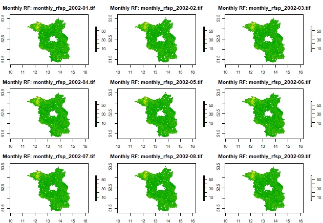
Plot 3x3 grid of monthly rasters as examples

# Get list of created rasters
raster_files <- list.files(output_dir, pattern = "monthly_rfsp_.*\\.tif$", full.names = TRUE)

# Check and plot up to 9 rasters
if (length(raster_files) > 0) {
  num_to_plot <- min(9, length(raster_files))
  selected_files <- raster_files[1:num_to_plot]

  # Set plotting layout
  par(mfrow = c(3, 3), mar = c(2, 2, 3, 4))

  for (i in seq_along(selected_files)) {
    r <- raster(selected_files[i])
    plot(r, main = paste0("Monthly RF: ", basename(selected_files[i])),
         col = terrain.colors(100))
  }

  par(mfrow = c(1, 1))  # Reset layout
} else {
  message("No raster files found for plotting.")
}

Create predictions with RFSI model

# Load required libraries
library(sp)
library(sf)
library(raster)
library(meteo)
library(data.table)
library(dplyr)

# Load input data and model
load("stfdf_2001-05.rda")
load("../models/RFSI_2001-05.rda")

# Define covariates
covariates <- c("GWD", "Lat", "Lon", "SLOPE", "ASP", "DEM", "LNF", "TPI", "TWI", "TRI",
                "PREC", "TEMP", "NDVI", "ET", "EVI")

# Extract and clean data from STFDF
GWD_df <- as.data.frame(stfdf)[, c("sp.ID", "time", covariates)]
GWD_df <- GWD_df[complete.cases(GWD_df), ]

# Prepare temporal information
time <- sort(unique(GWD_df$time))
days <- gsub("-", "", time, fixed = TRUE)

# Convert to clean dataframe for later use
newdata <- GWD_df %>% na.omit()

# Define years for processing
years_of_interest <- 2001:2005

# Loop through each year
for (year in years_of_interest) {

  message("Processing year: ", year)

  # Load test data
  test_data_file <- file.path(base_path, "project", "b_data_for_prediction",
                              paste0("data_for_pred_", year, "_v2.csv"))
  if (!file.exists(test_data_file)) {
    warning("Test data missing for ", year)
    next
  }

  data <- fread(test_data_file) %>% na.omit()

  # Convert test data to spatial object
  spatial_points_df <- SpatialPointsDataFrame(coords = data[, .(Lon, Lat)], data = data,
                                              proj4string = CRS("+proj=longlat +datum=WGS84"))

  # Order columns and remove redundant fields
  desired_order <- c("Date", "Lat", "Lon", "SLOPE", "ASP", "DEM", "LNF", "TPI", "TWI",
                     "TRI", "PREC", "TEMP", "NDVI", "ET", "EVI")
  rest <- setdiff(names(data), desired_order)
  data <- data[, c(desired_order, rest), with = FALSE]
  data <- data[, !names(data) %in% c("staid", "Lon.1", "Lat.1", "X", "Y", "optional"), with = FALSE]
  data <- na.omit(data)

  # Convert data to sf
  loc_sf <- st_as_sf(data, coords = c("Lon", "Lat"), crs = 4326)
  newdata_sf <- st_as_sf(newdata, coords = c("Lon", "Lat"), crs = 4326)
  loc_sf$Date <- as.Date(loc_sf$Date)
  newdata_sf$time <- as.Date(newdata_sf$time)

  # Compute nearest observations
  unique_dates <- unique(loc_sf$Date)
  nearest_obs_list <- list()

  for (current_date in unique_dates) {
    message("  Finding nearest observations for date: ", current_date)

    loc_day <- loc_sf[loc_sf$Date == current_date, ]
    newdata_day <- newdata_sf[newdata_sf$time == current_date, ]

    if (nrow(loc_day) == 0 || nrow(newdata_day) == 0) next

    nearest_obs <- meteo::near.obs(
      locations = loc_day,
      observations = newdata_day,
      obs.col = "GWD",
      n.obs = 100
    )

    nearest_obs_list[[as.character(current_date)]] <- nearest_obs
  }

  # Combine nearest observations
  nearest_obs_combined <- do.call(rbind, nearest_obs_list)
  nearest_obs_combined$date <- gsub("\\.\\d+$", "", rownames(nearest_obs_combined))
  rownames(nearest_obs_combined) <- NULL
  nearest_obs_combined <- nearest_obs_combined[, c("date", setdiff(names(nearest_obs_combined), "date"))]

  # Merge with spatial data
  merged_data <- cbind(st_drop_geometry(loc_sf), nearest_obs_combined)

  # Prepare for prediction
  merged_data <- merged_data[, !names(merged_data) %in% c("geometry", "Date")]

  # Predict using RFSI model
  message("  Predicting groundwater depth for ", year)
  predictions <- predict(rfsi_model, merged_data)
  loc_sf$Predictions <- predictions$prediction

  # Convert to dataframe for rasterization
  loc_df <- st_drop_geometry(loc_sf)
  coords <- st_coordinates(loc_sf)
  loc_df <- cbind(coords, loc_df)
  colnames(loc_df)[1:2] <- c("Lon", "Lat")

  # Save predictions as CSV
  output_csv <- file.path(base_path, "project", paste0(year, "_pred_rfsi.csv"))
  fwrite(loc_df, output_csv)

  # Load and project reference raster
  reference_raster <- raster(file.path(base_path, "project/brandenburg", "DEM.tif"))
  projected_raster <- projectRaster(reference_raster, crs = CRS("+proj=longlat +datum=WGS84"))

  # Create monthly rasters
  loc_df$Date <- as.Date(loc_df$Date)
  months <- unique(format(loc_df$Date, "%Y-%m"))
  output_dir <- file.path(base_path, "plot", "del")

  for (month in months) {
    message("  Creating raster for month: ", month)
    monthly_data <- loc_df[format(loc_df$Date, "%Y-%m") == month, ]

    sp_data <- SpatialPointsDataFrame(coords = monthly_data[, c("Lon", "Lat")],
                                      data = data.frame(Predictions = monthly_data$Predictions),
                                      proj4string = CRS("+proj=longlat +datum=WGS84"))

    monthly_raster <- rasterize(sp_data, projected_raster, field = "Predictions")
    output_file <- file.path(output_dir, paste0("monthly_rfsi_", month, ".tif"))

    writeRaster(monthly_raster, filename = output_file, format = "GTiff", overwrite = TRUE)
  }

  message("Completed year: ", year)
}

message("All RFSI predictions completed successfully.")

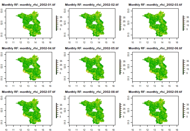
Plot 3x3 grid of monthly rasters as examples

# Get list of created rasters
raster_files <- list.files(output_dir, pattern = "monthly_rfsi_.*\\.tif$", full.names = TRUE)

# Check and plot up to 9 rasters
if (length(raster_files) > 0) {
  num_to_plot <- min(9, length(raster_files))
  selected_files <- raster_files[1:num_to_plot]

  # Set plotting layout
  par(mfrow = c(3, 3), mar = c(2, 2, 3, 4))

  for (i in seq_along(selected_files)) {
    r <- raster(selected_files[i])
    plot(r, main = paste0("Monthly RF: ", basename(selected_files[i])),
         col = terrain.colors(100))
  }

  par(mfrow = c(1, 1))  # Reset layout
} else {
  message("No raster files found for plotting.")
}