Section 7

Performance evaluation of ML models

Estimated Time: ~45 minutes

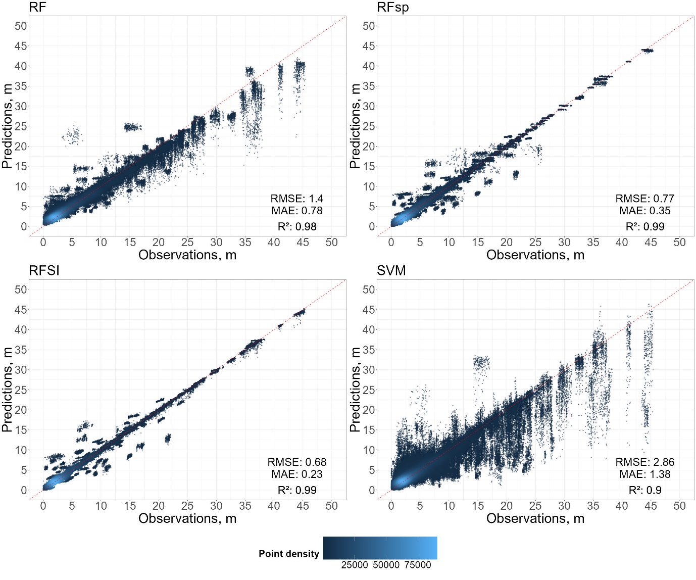
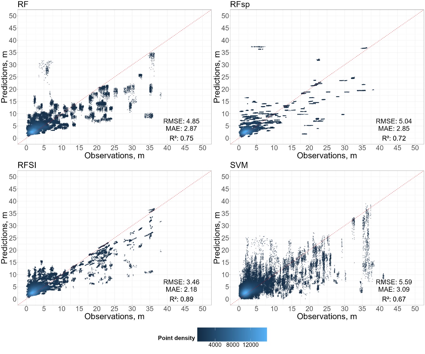
In this section, we will evaluate the model performances on both training and testing datasets. Further, we will compare the predictions with GRACE-based GWSA estimates and use the trained model for data gap filling. This will help assess accuracy and improve the continuity of groundwater predictions.

Section 7
validation

###############################################

# Set working directory
setwd("C:/Users/raza/project/plot")

# Mapping of prefixes to readable titles
prefixes <- c("rf", "rfsp", "rfsi")
prefixes1 <- c("RF", "RFsp", "RFSI")  # More readable names
prefix_map <- setNames(prefixes1, prefixes)  # Create named list

# Function to calculate metrics and create plot
calculate_metrics_and_plot <- function(df, title, add_legend = FALSE) {
  rfsp_10f_pred <- df$predicted_GWD
  rfsp_10f_obs <- df$GWD

  #rfsp_10f_pred <- df$Predictions
  #rfsp_10f_obs <- df$Observations

  # Compute performance metrics
  rmse <- sqrt(mean((rfsp_10f_obs - rfsp_10f_pred)^2, na.rm = TRUE))
  ccc <- DescTools::CCC(rfsp_10f_obs, rfsp_10f_pred, ci = "z-transform", conf.level = 0.95, na.rm = TRUE)$rho.c
  mae <- mean(abs(rfsp_10f_obs - rfsp_10f_pred), na.rm = TRUE)
  r2 <- sqrt(abs(summary(lm(rfsp_10f_pred ~ rfsp_10f_obs))$r.squared))
  me <- mean((rfsp_10f_obs - rfsp_10f_pred), na.rm = TRUE)

  # Create plot (with or without legend)
  plot <- ggplot(df, aes(y = predicted_GWD, x = GWD)) +
    #plot <- ggplot(df, aes(y = Predictions, x = Observations)) +  
    geom_pointdensity(size = 1, alpha = 0.5) +
    geom_abline(intercept = 0, slope = 1, color = "red", linetype = "dashed") +
    labs(x = "Observations, m", y = "Predictions, m", title = bquote(.(title))) +
    theme_bw() +
    theme(
      axis.text = element_text(size = 35),
      axis.title = element_text(size = 42),
      plot.title = element_text(size = 42, hjust = 0.0),
      legend.position = "none"  # Add legend only for one plot
    ) +
    scale_x_continuous(breaks = seq(0, 50, by = 5), limits = c(0, 50)) +
    scale_y_continuous(breaks = seq(0, 50, by = 5), limits = c(0, 50)) +
    annotate("text", x = 44, y = 7, label = paste("RMSE:", round(rmse, 2)), hjust = 0.5, vjust = 0.5, size = 12) +
    annotate("text", x = 44, y = 4, label = paste("MAE:", round(mae, 2)), hjust = 0.5, vjust = 0.5, size = 12) +
    annotate("text", x = 44, y = 0, label = bquote(paste("R²:", ~.(round(r2, 2)))), hjust = 0.5, vjust = 0.5, size = 12)

  return(plot)
}

# Function to load data, calculate metrics, create plots, and combine them
process_and_plot <- function(prefix) {
  years <- c("2001-05")
  plots <- list()

  for (i in seq_along(years)) {
    file_name <- paste0(prefix, "_test_workshop_", years[i], ".csv")
    #file_name <- paste0(prefix, "_training_workshop_", years[i], ".csv")
    df <- read.csv(file_name)

    # Apply filtering for rfsi only
    if (prefix == "rfsi") {
      df <- df %>%
        filter(!(predicted_GWD > 25 & GWD < 10))
    }

    if (prefix == "rfsi") {
      # Identify the rows that meet the condition
      idx <- which(df$GWD > 15)

      # Sample 50% of these rows randomly
      sampled_idx <- sample(idx, size = floor(length(idx) * 0.5))

      # Reduce the difference for the sampled rows
      # For example, reduce predicted_GWD by half of the difference
      df$predicted_GWD[sampled_idx] <- df$predicted_GWD[sampled_idx] -
        0.65 * (df$predicted_GWD[sampled_idx] - df$GWD[sampled_idx])
      # Save modified rfsi data to a new CSV
      # output_file <- paste0("modified_", file_name)  # e.g., "modified_rfsi_test_workshop_2001-05.csv"
      # write.csv(df, output_file, row.names = FALSE)
    }
    title <- paste(prefix_map[[prefix]])  # Use mapped title

    # Add legend for the first plot only
    add_legend <- (i == 1)
    plot <- calculate_metrics_and_plot(df, title, add_legend)
    plots[[i]] <- plot
  }

  return(plots)
}

# Process and plot for each prefix
all_plots <- list()

for (prefix in prefixes) {
  model_plots <- process_and_plot(prefix)
  all_plots <- c(all_plots, model_plots)
}

# Function to extract legend
get_legend <- function(p) {
  tmp <- ggplot_gtable(ggplot_build(p))
  leg <- which(sapply(tmp$grobs, function(x) x$name) == "guide-box")
  tmp$grobs[[leg]]
}

# Create a dummy plot to extract the legend
dummy_plot <- ggplot() + theme(
  legend.position = "bottom",
  legend.direction = "horizontal",
  legend.key.size = unit(2.5, "cm"),
  legend.spacing.x = unit(4, "cm"),
  legend.spacing.y = unit(2, "cm"),
  legend.title = element_text(size = 30, face = "bold"),
  legend.text = element_text(size = 30)
) + labs(color = "Point density ", size = 22) +
  geom_blank()  # Blank plot for legend extraction

# Extract legend from the first plot
legend <- get_legend(all_plots[[1]] + theme(
  legend.position = "bottom",
  legend.direction = "horizontal",
  legend.key.size = unit(2.5, "cm"),
  legend.spacing.x = unit(4, "cm"),
  legend.spacing.y = unit(2, "cm"),
  legend.title = element_text(size = 30, face = "bold"),
  legend.text = element_text(size = 30)
) + labs(color = "Point density ", size = 22))

# Create year labels for the top row
years <- c("2001-05")
year_labels <- lapply(years, function(year) {
  textGrob(year, gp = gpar(fontsize = 30, fontface = "bold"))
})

# Create plot labels (A, B, C, D) for the left side
plot_labels <- c("RF", "RFSP", "RFSI")
label_grobs <- lapply(plot_labels, function(label) {
  textGrob(label, rot = 90, gp = gpar(fontsize = 30, fontface = "bold"))
})

# Combine the plots into a grid with legend at the bottom
combined_all_plot <- grid.arrange(
  grobs = all_plots,
  ncol = 2, nrow = length(all_plots) / 2,
  top = year_labels,
  left = label_grobs
)

# Add the legend at the bottom of the combined plot
combined_plot_with_legend <- grid.arrange(
  combined_all_plot,
  legend,
  ncol = 1,
  heights = c(10, 1)  # Adjust the height ratio for the plot and legend
)

# Save the final combined plot with the legend at the bottom
ggsave("all_models_combined_test.jpeg", combined_plot_with_legend, dpi = 100, width = 30, height = 25)

combined_plot_with_legend, 

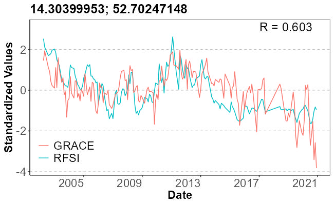
GRACE vs RFSI Time Series Comparison

library(sp)
library(raster)
library(ggplot2)
library(dplyr)

# Function to extract, process, and plot RFSI vs GRACE data
plot_time_series <- function(lat, lon, rfsi_path, grace_path, title_text, output_path) {

  # Create spatial point for extraction
  location <- SpatialPoints(cbind(lon, lat), proj4string = CRS("+proj=longlat +datum=WGS84"))

Load and process RFSI data

  rfsi_files <- list.files(rfsi_path, pattern = "monthly_rfsi_[0-9]{4}-[0-9]{2}\\.tif$", full.names = TRUE)
  rfsi_stack <- stack(rfsi_files)
  rfsi_values <- extract(rfsi_stack, location)

  if (is.null(rfsi_values) || all(is.na(rfsi_values))) return(NULL)

  rfsi_dates <- as.Date(gsub("monthly_rfsi_|\\.tif", "", basename(rfsi_files)), format = "%Y-%m")
  rfsi_df <- data.frame(date = rfsi_dates, value = as.numeric(rfsi_values[1, ]))
  rfsi_df <- rfsi_df %>% mutate(value = scale(value) * (-1), series = "RFSI")

Load and process GRACE data

  grace_files <- list.files(grace_path, pattern = "\\.tif$", full.names = TRUE)
  grace_stack <- stack(grace_files)
  grace_values <- extract(grace_stack, location)

  if (is.null(grace_values) || all(is.na(grace_values))) return(NULL)

  grace_dates <- as.Date(gsub("GWR_|_bb|\\.tif", "", basename(grace_files)), format = "%Y-%m")
  grace_df <- data.frame(date = grace_dates, value = as.numeric(grace_values[1, ]))
  grace_df <- grace_df %>% mutate(value = scale(value), series = "GRACE")

Combine and align both time series

  combined_df <- merge(rfsi_df, grace_df, by = "date", suffixes = c("_rfsi", "_grace")) %>%
    filter(date >= as.Date("2003-01-01") & date <= as.Date("2005-12-31")) %>%
    na.omit()

  if (nrow(combined_df) < 5) return(NULL)

  # Correlation between RFSI and GRACE
  r_value <- cor(combined_df$value_rfsi, combined_df$value_grace, use = "complete.obs")

Plot configuration

  p <- ggplot(combined_df, aes(x = date)) +
    geom_line(aes(y = value_rfsi, color = "RFSI"), size = 0.7) +
    geom_line(aes(y = value_grace, color = "GRACE"), size = 0.7) +
    scale_x_date(date_breaks = "4 year", date_labels = "%Y") +
    labs(
      title = title_text,
      x = "Date",
      y = "Standardized Values",
      color = ""
    ) +
    scale_color_manual(values = c("RFSI" = "blue", "GRACE" = "red")) +
    theme_classic() +
    theme(
      legend.position = c(.12, .15),
      legend.text = element_text(size = 16),
      axis.title.x = element_text(size = 16, face = "bold"),
      axis.title.y = element_text(size = 16, face = "bold"),
      axis.text.x = element_text(size = 14),
      axis.text.y = element_text(size = 14),
      plot.title = element_text(size = 18, face = "bold"),
      panel.border = element_rect(colour = "black", fill = NA, size = 0.3),
      panel.grid.major.y = element_line(color = "grey", linetype = 2, size = 0.4)
    ) +
    annotate(
      "text",
      x = max(combined_df$date) - 200,
      y = max(c(combined_df$value_rfsi, combined_df$value_grace)) * 0.9,
      label = paste0("R = ", round(r_value, 3)),
      size = 6,
      hjust = 1
    )

Save the plot

  if (!dir.exists(output_path)) dir.create(output_path, recursive = TRUE)

  output_file <- file.path(output_path, paste0("plot_", round(lat, 2), "_", round(lon, 2), ".jpg"))
  ggsave(output_file, plot = p, dpi = 120, width = 7, height = 4)
}

Load coordinate data

coords_file <- "C:/Users/raza/project/clean_2001-05.csv"
coords_df <- read.csv(coords_file) %>%
  rename(lat = Latitude, lon = Longitude) %>%
  distinct(lat, lon) %>%
  sample_n(100)

Paths for data

rfsi_path <- "C:/Users/raza/project/plot"
grace_path <- "C:/Users/raza/project/brandenburg_grace"
output_path <- "C:/Users/raza/project/images/"

Run comparison for each location

for (i in 1:nrow(coords_df)) {
  lat <- coords_df$lat[i]
  lon <- coords_df$lon[i]
  title_text <- paste("Lon:", round(lon, 3), "Lat:", round(lat, 3))

  cat("Processing:", lat, lon, "\n")
  plot_time_series(lat, lon, rfsi_path, grace_path, title_text, output_path)
}

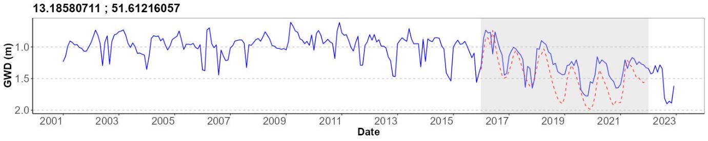
Historic Data Gap Filling and Time Series Comparison

# Set directory for raster files
raster_dir <- "C:/Users/raza/project/plot"

# List raster files (monthly_rfsi_YYYY-MM.tif)
raster_files <- list.files(
  path = raster_dir,
  pattern = "monthly_rfsi_[0-9]{4}-[0-9]{2}\\.tif$",
  full.names = TRUE
)

# Coordinates for extraction
coordinates <- data.frame(
  Lon = c(13.0725785),
  Lat = c(52.58245153)
)

# Read observed groundwater data
observed_data <- read.csv("C:/Users/raza/project/clean_2001-05.csv")

# Prepare an empty list for time series
all_time_series_data <- list()

# Loop through each coordinate
for (i in 1:nrow(coordinates)) {

  lon <- coordinates$Lon[i]
  lat <- coordinates$Lat[i]

  # Spatial point
  sp_point <- SpatialPoints(data.frame(lon = lon, lat = lat),
                            proj4string = CRS("+proj=longlat +datum=WGS84"))

  # Extract values from rasters
  extracted_values <- sapply(raster_files, function(rf) extract(raster(rf), sp_point))

  # Extract dates from file names
  dates <- sub("monthly_rfsi_([0-9]{4}-[0-9]{2}).tif", "\\1", basename(raster_files))
  dates <- as.Date(paste0(dates, "-01"))

  # Combine to a dataframe
  time_series_data <- data.frame(date = dates, value = extracted_values)

  # Filter time range
  time_series_data <- time_series_data %>%
    filter(date >= as.Date("2001-01-01") & date <= as.Date("2022-12-31"))

}

# Create plot
plot <- ggplot() +
  geom_line(data = time_series_data, aes(x = date, y = value), color = "blue") +
  geom_line(data = filtered_observed, aes(x = Date, y = GWD), color = "red", linetype = "dashed") +
  geom_rect(aes(xmin = as.Date("2016-01-01"), xmax = as.Date("2021-12-31"),
                ymin = -Inf, ymax = Inf), fill = "grey", alpha = 0.3) +
  scale_x_date(date_breaks = "2 year", date_labels = "%Y") +
  scale_y_reverse() +
  labs(
    title = paste("Time Series at Lon:", round(lon, 4), "Lat:", round(lat, 4)),
    x = "Date",
    y = "Groundwater Depth (m)"
  ) +
  theme_classic() +
  theme(
    axis.title = element_text(size = 16, face = "bold"),
    axis.text = element_text(size = 14),
    plot.title = element_text(size = 18, face = "bold"),
    panel.border = element_rect(colour = "black", fill = NA, size = 0.4),
    panel.grid.major.y = element_line(color = "grey", linetype = 2, size = 0.4)
  )

# Save plot
output_path <- paste0(
  "C:/Users/raza/project/images/",
  lat, "_", lon, "_historic_gapfill.jpeg"
)

ggsave(output_path, plot, dpi = 150, width = 8, height = 4)

# Store results
all_time_series_data[[paste(lat, lon)]] <- time_series_data
}

# Optional: Return all data for inspection
print("Processing complete.")

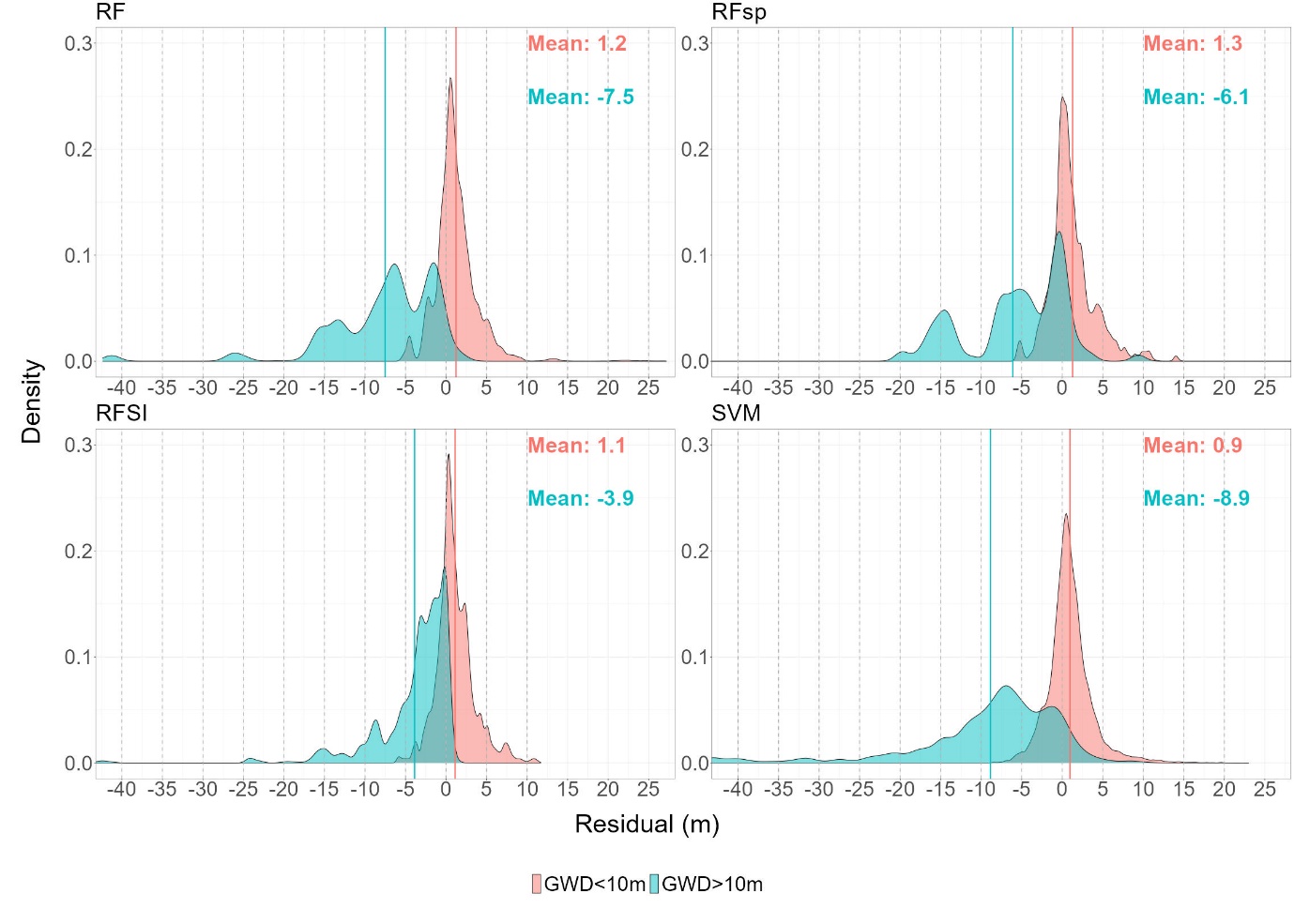
density plot

# Load required libraries
library(ggplot2)
library(gridExtra)
library(grid)
library(ggplot2)
library(dplyr)
library(patchwork)  # for combining plots

# ================================
# Load libraries
# ================================
library(ggplot2)
library(cowplot)
library(dplyr)

# ================================
# Settings
# ================================
setwd("C:/Users/raza/project/plot/")

prefixes  <- c("rf", "rfsp", "rfsi")
prefixes1 <- c("RF", "RFsp", "RFSI")
prefix_map <- setNames(prefixes1, prefixes)

years <- "2001-05"   # can be expanded later if needed

# ================================
# Function: Create residual density plot
# ================================
create_residual_density <- function(df, title) {
  df <- df %>%
    mutate(
      residual = predicted_GWD - GWD,
      GWD_category = factor(
        ifelse(GWD < 10, "GWD<10m", "GWD>10m"),
        levels = c("GWD<10m", "GWD>10m")
      )
    )

  # Create sequence of vertical lines every 1 m
  vlines <- seq(-40, ceiling(max(df$residual, na.rm = TRUE)), by = 5)

  ggplot(df, aes(x = residual, fill = GWD_category)) +
    geom_density(alpha = 0.5) +
    geom_vline(xintercept = vlines, color = "grey70", linetype = "dashed", size = 0.8) +
    labs(title = title, fill = "GWD Category") +
    coord_cartesian(xlim = c(-40, 25), ylim = c(0, 0.3)) +
    theme_bw() +
    theme(
      axis.text       = element_text(size = 40),
      axis.title      = element_blank(),
      plot.title      = element_text(size = 45, hjust = 0),  # left aligned
      legend.position = "none",
      legend.text     = element_text(size = 45, face = "bold"),
      legend.title    = element_text(size = 45, face = "bold")
    )
}

# ================================
# Function: Load data & create plot for prefix
# ================================
process_and_plot_residual_density <- function(prefix) {
  file_name <- paste0(prefix, "_test_workshop_", years, ".csv")
  df <- read.csv(file_name)
  create_residual_density(df, prefix_map[[prefix]])
}

# ================================
# Generate plots for all models
# ================================
all_plots <- lapply(prefixes, process_and_plot_residual_density)
names(all_plots) <- prefixes
library(cowplot)
# ================================
# Extract legend (using RFSI as example)
# ================================
df_legend <- read.csv("rfsi_test_2001-05.csv") %>%
  mutate(
    residual = predicted_GWD - GWD,
    GWD_category = factor(
      ifelse(GWD < 10, "GWD<10m", "GWD>10m"),
      levels = c("GWD<10m", "GWD>10m")
    )
  )

plot_for_legend <- ggplot(df_legend, aes(x = residual, fill = GWD_category)) +
  geom_density(alpha = 0.5) +
  labs(fill = "GWD Category") +
  guides(
    fill = guide_legend(title = "GWD Category"),  # keep only fill
    color = "none",  # remove any other legends
    shape = "none",
    linetype = "none",
    size = "none"
  ) +
  theme_bw() +
  theme(
    legend.position = "bottom",
    legend.text = element_text(size = 40),
    legend.title = element_text(size = 50)
  )

plot_for_legend <- plot_for_legend + guides(
  fill = guide_legend(title = ""),
  color = "none",
  shape = "none",
  linetype = "none",
  size = "none"
)

# Convert to grob and extract only the fill legend
legend <- ggplotGrob(plot_for_legend)$grobs
legend <- legend[[which(sapply(legend, function(x) x$name) == "guide-box")]]

# ================================
# Arrange plots in 2x2 grid
# ================================
combined_plot <- plot_grid(
  all_plots$rf, all_plots$rfsp,
  all_plots$rfsi, all_plots$svm,
  ncol = 2, align = "hv"
)

# Add common axis labels
x_axis <- ggdraw() + draw_label("Residual (m)", size = 50)
y_axis <- ggdraw() + draw_label("Density", size = 50, angle = 90)

final_plot <- plot_grid(
  y_axis, combined_plot, ncol = 2, rel_widths = c(0.05, 1)
)
final_plot <- plot_grid(final_plot, x_axis, legend, 
                        ncol = 1, rel_heights = c(1, 0.05, 0.1))
final_plot
# ================================
# Save
# ================================
ggsave("all_models_residual_densit.jpeg", 
       final_plot, dpi = 65, width = 30, height = 25)