Section 2

Curate and harmonize groundwater time series; identify and address quality issues

Estimated Time: ~1hr

In this section, we explore and prepare the groundwater monitoring data set. We then conduct a data quality assessment to determine the total number of wells to be used in this study to exclude anthropogenic and extreme climate conditions. Several criteria were applied to this initial selection process: (1) the consistency of data at each well; (2) the observational uncertainty related to the head values in the well database (RMSE =< 0.25m); and (3) continuous functionality of the well.

Please make sure that you have installed all the packages mentioned in the previous sections.

Curate and harmonize groundwater time series; identify and address quality issues

Identify CSV files starting from year 2000 and optionally remove others

folder_path <- "C:/Users/raza/project/ObsWell_based_data"
csv_files <- list.files(path = folder_path, pattern = "\\.csv$", full.names = TRUE)

num_files_meeting_condition <- 0

for (csv_file in csv_files) {
  data <- read.csv(csv_file)
  first_date <- dmy(data$Date[1])

  if (!is.na(first_date) && year(first_date) >= 2000) {
    num_files_meeting_condition <- num_files_meeting_condition + 1
    cat("File:", basename(csv_file), "\n")
    print(head(data$Date, 5))
    # Remove file if needed
    # unlink(csv_file)
  }
}

cat("Number of files meeting condition:", num_files_meeting_condition, "\n")

Extract yearly data and add well ID

source_folder <- folder_path
destination_folder <- "C:/Users/raza/project/monthly_data"
dir_create(destination_folder)

specific_years <- 2001:2005

filter_and_add_filename <- function(data, year, filename) {
  data <- data %>%
    mutate(Date = dmy(Date)) %>%
    filter(year(Date) == year) %>%
    mutate(ID = filename)
  return(data)
}

csv_files <- dir_ls(source_folder, regexp = "\\.csv$")

for (yr in specific_years) {
  data_list <- list()
  for (csv_file in csv_files) {
    data <- read.csv(csv_file, stringsAsFactors = FALSE)
    filename <- substr(tools::file_path_sans_ext(basename(csv_file)), 1, 8)
    data_list[[filename]] <- filter_and_add_filename(data, yr, filename)
  }

  combined_data <- bind_rows(data_list)
  write.csv(combined_data, paste0(destination_folder, "/", yr, ".csv"), row.names = FALSE)
  cat("Year", yr, "data saved.\n")
}

Merge coordinates by Well ID

coordinate_file <- "C:/Users/raza/project/example/stammdaten_2023_07.csv"
coordinates_data <- read.csv(coordinate_file, stringsAsFactors = FALSE, fileEncoding = "UTF-8")

mean_monthly_folder <- "C:/Users/raza/project/mean_monthly_data"
file_list <- list.files(mean_monthly_folder, pattern = "\\.csv$", full.names = TRUE)

for (file in file_list) {
  well_data <- read.csv(file, stringsAsFactors = FALSE)
  merged_data <- merge(well_data, coordinates_data, by = "ID", all.x = TRUE)
  write.csv(merged_data, paste0("merged_", basename(file)), row.names = FALSE)
}

Calculate mean monthly GWL

monthly_files <- list.files(destination_folder, pattern = "\\.csv$", full.names = TRUE)
monthly_mean_list <- list()

for (file in monthly_files) {
  data <- read.csv(file)
  data$Date <- as.Date(data$Date)
  data$Month <- format(data$Date, "%Y-%m")

  monthly_mean <- data %>%
    group_by(ID, Month) %>%
    summarize(Mean_GWL = mean(GWL, na.rm = TRUE), .groups = "drop")

  monthly_mean_list[[basename(file)]] <- monthly_mean
  write.csv(monthly_mean, gsub(".csv", "_monthly_mean.csv", file), row.names = FALSE)
}

Clean stations with missing months and transpose for PCA

clean_folder <- "C:/Users/raza/project/mean_monthly_data"

file_list <- list.files(clean_folder, pattern = "*.csv", full.names = TRUE)

for (file in file_list) {
  data <- read.csv(file)
  data$Date <- as.yearmon(data$Month, "%Y-%m")

  ids_to_remove <- data %>%
    group_by(ID) %>%
    summarize(Num_Unique_Months = n_distinct(Date)) %>%
    filter(Num_Unique_Months < 12) %>%
    pull(ID)

  data_filtered <- data %>% filter(!ID %in% ids_to_remove)

  clean_filename <- paste0("clean_", gsub("[^0-9]", "", basename(file)), ".csv")
  write.csv(data_filtered, clean_filename, row.names = FALSE)

  data_transposed <- pivot_wider(data_filtered, names_from = ID, values_from = Mean_GWL)
  data_transposed <- data_transposed %>% select(where(~ !any(is.na(.))))

  transposed_filename <- paste0("transposed_", gsub("[^0-9]", "", basename(file)), ".csv")
  write.csv(data_transposed, transposed_filename, row.names = TRUE)
}

PCA Analysis

data <- read.csv("transposed_2001-05.csv")
data_num <- data[, -1]  # remove first column if necessary
data_num <- sapply(data_num, as.numeric)
data_num[is.na(data_num)] <- mean(data_num, na.rm = TRUE)

z_scaled_data <- scale(data_num)
pca_result <- prcomp(z_scaled_data)

summary(pca_result)

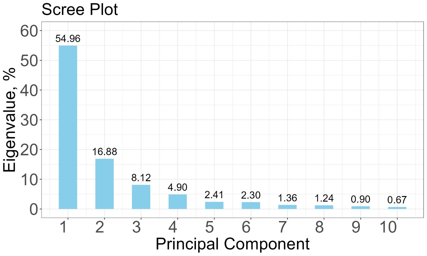
# Scree plot
eigenvalues <- (pca_result$sdev)^2 / sum((pca_result$sdev)^2) * 100
eig_df <- data.frame(Dimension = 1:length(eigenvalues), Eigenvalue = eigenvalues)
eig_df_sub <- head(eig_df, 10)

p <- ggplot(eig_df_sub, aes(x = Dimension, y = Eigenvalue)) +
  geom_bar(stat = "identity", fill = "skyblue", width = 0.5) +
  geom_text(aes(label = round(Eigenvalue, 2)), vjust = -0.5, size = 6) +
  labs(title = "Scree Plot", x = "Principal Component", y = "Variance (%)") +
  theme_bw() +
  theme(axis.text = element_text(size = 28), axis.title = element_text(size = 28), plot.title = element_text(size = 28))
ggsave("scree_plot_1.jpg", plot = p, width = 10, height = 6, units = "in", dpi = 200)

# Save PCA results
write.csv(pca_result$x, "scores_2001-05.csv")
write.csv(pca_result$rotation, "loadings_2001-05.csv")

Reference Hydrograph & Residuals

pc_scores <- as.data.frame(pca_result$x)
regression_data <- cbind(data_num, pc_scores)
reference_hydrographs <- data.frame()
residuals_data <- data

for (well_col in 1:ncol(data_num)) {
  lm_result <- lm(data_num[, well_col] ~ PC1 + PC2 + PC3 + PC4, data = regression_data)
  reference <- predict(lm_result)

  reference_hydrographs <- rbind(reference_hydrographs, data.frame(
    Well = colnames(data_num)[well_col],
    Reference_Hydrograph = reference
  ))

  residuals_data[, well_col] <- data_num[, well_col] - reference
}

write.csv(reference_hydrographs, "reference_hydrographs.csv")
write.csv(residuals_data, "residuals_data.csv")

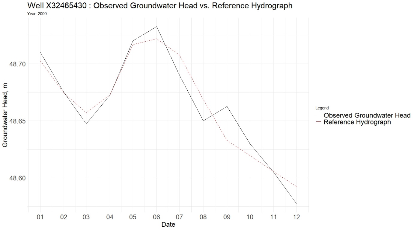
Plot Observed vs Reference Hydrograph

well_name <- "X32465430"
plot_data <- data.frame(
  Date = as.Date(data$Month),
  Groundwater_Head = data[[well_name]],
  Reference_Hydrograph = reference_hydrographs$Reference_Hydrograph[reference_hydrographs$Well == well_name]
)

ggplot(plot_data, aes(x = Date)) +
  geom_line(aes(y = Groundwater_Head, color = "Observed"), size = 1) +
  geom_line(aes(y = Reference_Hydrograph, color = "Reference"), size = 1, linetype = "dashed") +
  labs(title = paste("Well", well_name), x = "Year", y = "Groundwater Head") +
  scale_color_manual(values = c("Observed" = "black", "Reference" = "red")) +
  theme_bw()

Calculate RMSE

well_rmses <- data.frame(Well = colnames(data_num), RMSE = NA)

for (i in seq_along(well_rmses$Well)) {
  obs <- data_num[, i]
  ref <- reference_hydrographs$Reference_Hydrograph[reference_hydrographs$Well == well_rmses$Well[i]]
  well_rmses$RMSE[i] <- sqrt(mean((obs - ref)^2))
}

ranked_wells <- well_rmses[order(well_rmses$RMSE), ]
write.csv(well_rmses, "RMSE_2001-05.csv")

plots with RMSE > 0.25m

setwd("C:/Users/raza/project")
data <- read.csv("total.csv")

plot <- ggplot(data_melt, aes(x = factor(year), y = value, color = variable, group = variable)) +
  geom_line(size = 1.2) +  # Line plot with increased line width
  labs(title = "",
       x = "Year",
       y = "Number of wells") +  
  theme_bw() +  
  theme(legend.position = "bottom",
        axis.text.x = element_text(angle = 0, hjust = 1, size = 16, face = "bold"),  
        axis.text.y = element_text(size = 16, face = "bold"),
        axis.title = element_text(size = 18),
        legend.title = element_blank(),  
        legend.text = element_text(size = 14, face = "bold"),
        plot.title = element_text(size = 14, face = "bold")) +  
  scale_color_manual(values = c("Total.Wells" = "#E41A1C", "Complete.Data" = "#377EB8", 
                                "RMSE...0.25m" = "darkgreen", "RMSE....0.25m" = "darkgoldenrod", 
                                "Missing.Data" = "orange"),
                     labels = c("Total Wells", 
                                "Wells with complete data", 
                                "RMSE <= 0.25m", 
                                "Wells with missing data", 
                                "RMSE > 0.25m")) +
  scale_x_discrete(breaks = seq(2001, 2005, by = 1))  +  
  geom_vline(xintercept = c("2001", "2005"), 
             linetype = "dashed", color = "black", size = 0.45) +  
  guides(color = guide_legend(nrow = 2))

plot

# Save the plot as a PNG file
ggsave("total_v2.png", plot = plot, width = 10, height = 7, dpi = 100)