Section 2

Supervised learning with labeled remote sensing data

Estimated Time: ~25 minutes

Make sure that you have all installed libraries presented in section 1 of the practical part.

Run the SL.ipynb file.

Import the Python frameworks we need for this tutorial.

# torch implementation
import os
import torch
import torchvision
import torchvision.transforms as transforms
from torchvision.datasets import ImageFolder
from torch.utils.data import DataLoader, random_split, Subset
import torchvision.models as models
from torchvision.models import resnet18
import torch.nn.functional as F
from torchsummary import summary
from torch import Tensor
from torch import nn
from torchvision.transforms import InterpolationMode
from torchvision import transforms, datasets
import torch.optim as optim
import random

# image processing and disply
import matplotlib.pyplot as plt
import numpy as np
import time
from PIL import ImageOps, ImageFilter, Image, ImageDraw, ImageFont

# warnings
import warnings
warnings.filterwarnings("ignore")
warnings.filterwarnings("ignore", module = "matplotlib\..*")

Check the GPU

if torch.cuda.is_available():
    print("CUDA version:", torch.version.cuda)
    print("GPU Name:", torch.cuda.get_device_name(0))
else:
    print("No GPU available for CUDA.")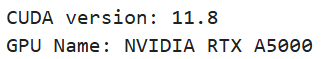

# Paths
data_dir = 'C:/Workshop/dataset_SL'  # Your dataset path

# Augmentations for training
train_transform = transforms.Compose([
    transforms.Resize((150, 150)),
    transforms.RandomHorizontalFlip(),
    transforms.RandomRotation(10),
    transforms.ColorJitter(brightness=0.2, contrast=0.2, saturation=0.2, hue=0.05),
    transforms.RandomResizedCrop(128, scale=(0.8, 1.0)),
    transforms.ToTensor(),
    transforms.Normalize((0.5,), (0.5,))
])

# No augmentation for validation/test, just resizing and normalization
test_transform = transforms.Compose([
    transforms.Resize((128, 128)),
    transforms.ToTensor(),
    transforms.Normalize((0.5,), (0.5,))
])

# Full dataset using one transform first (we'll reassign transforms later)
full_dataset = datasets.ImageFolder(root=data_dir, transform=test_transform)

# Split sizes
train_size = int(0.80 * len(full_dataset))
val_size = int(0.10 * len(full_dataset))
test_size = len(full_dataset) - train_size - val_size

# Split
trainset, valset, testset = random_split(full_dataset, [train_size, val_size, test_size])

# Assign transform to train split manually
trainset.dataset.transform = train_transform
valset.dataset.transform = test_transform
testset.dataset.transform = test_transform

# DataLoaders
trainloader = DataLoader(trainset, batch_size=64, shuffle=True, num_workers=4)
valloader = DataLoader(valset, batch_size=64, shuffle=False, num_workers=4)
testloader = DataLoader(testset, batch_size=64, shuffle=False, num_workers=4)

# Print splits
print(f"Trainset: {len(trainset)}, Valset: {len(valset)}, Testset: {len(testset)}")

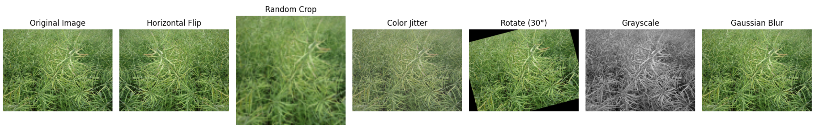
Let's visualise different data augmentation techniques

# Path to your dataset
data_dir = 'C:/Workshop/dataset_SL'

# Load dataset without augmentation
dataset = datasets.ImageFolder(root=data_dir, transform=transforms.ToTensor())

# Select a random image from the dataset
idx = random.randint(0, len(dataset) - 1)
img_tensor, _ = dataset[idx]
img = transforms.ToPILImage()(img_tensor)

# Define augmentations
augmentations = {
    "Original Image": lambda x: x,
    "Horizontal Flip": transforms.RandomHorizontalFlip(p=1),
    "Random Crop": transforms.RandomResizedCrop((100, 100), scale=(0.8, 1.0)),
    "Color Jitter": transforms.ColorJitter(0.4, 0.4, 0.4, 0.1),
    "Rotate (30°)": transforms.RandomRotation(30),
    "Grayscale": transforms.Grayscale(num_output_channels=3),
    "Gaussian Blur": transforms.GaussianBlur(5, sigma=(0.1, 2.0)),
}

# Apply and plot
fig, axes = plt.subplots(1, len(augmentations), figsize=(18, 4))
for ax, (name, aug) in zip(axes, augmentations.items()):
    aug_img = aug(img)
    ax.imshow(aug_img)
    ax.set_title(name)
    ax.axis("off")

plt.tight_layout()
plt.show()

from collections import Counter

def class_distribution(dataset):
    """Calculate the class distribution in the dataset."""
    # Get the labels from the dataset
    labels = [dataset[i][1] for i in range(len(dataset))]
    # Count occurrences of each class
    count = Counter(labels)

    # Calculate proportions
    total = sum(count.values())
    proportions = {k: v / total for k, v in count.items()}

    return proportions

# Calculate and print the class distributions for each dataset
train_distribution = class_distribution(trainset)
val_distribution = class_distribution(valset)
test_distribution = class_distribution(testset)

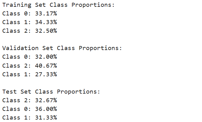
print("Training Set Class Proportions:")
for label, proportion in train_distribution.items():
    print(f"Class {label}: {proportion:.2%}")

print("\nValidation Set Class Proportions:")
for label, proportion in val_distribution.items():
    print(f"Class {label}: {proportion:.2%}")

print("\nTest Set Class Proportions:")
for label, proportion in test_distribution.items():
    print(f"Class {label}: {proportion:.2%}")

Load pre-trained ResNet18 model

model = models.resnet18(pretrained=True)

# Modify the final fully connected layer to match the number of classes in your dataset
num_classes = 3  # Adjust as per your dataset
model.fc = nn.Linear(model.fc.in_features, num_classes)

# Move the model to the appropriate device (GPU or CPU)
device = torch.device('cuda' if torch.cuda.is_available() else 'cpu')
model = model.to(device)

# Define the criterion and optimizer
criterion = nn.CrossEntropyLoss()
optimizer = optim.Adam(model.parameters(), lr=0.001)

# Variables to store training history
train_losses = []
val_losses = []
train_accuracies = []
val_accuracies = []
best_accuracy = 0
best_epoch = 0

# Training loop
num_epochs = 25
for epoch in range(num_epochs):
    model.train()
    running_loss = 0.0
    correct_train = 0
    total_train = 0

    # Train on training set
    for inputs, labels in trainloader:  # Assume trainloader is defined elsewhere
        inputs, labels = inputs.to(device), labels.to(device)

        optimizer.zero_grad()

        outputs = model(inputs)
        loss = criterion(outputs, labels)

        loss.backward()
        optimizer.step()

        running_loss += loss.item()

        _, predicted = torch.max(outputs.data, 1)
        total_train += labels.size(0)
        correct_train += (predicted == labels).sum().item()

    # Calculate training loss and accuracy
    train_loss = running_loss / len(trainloader)
    train_accuracy = 100 * correct_train / total_train
    train_losses.append(train_loss)
    train_accuracies.append(train_accuracy)

    # Validation loop
    model.eval()
    running_val_loss = 0.0
    correct_val = 0
    total_val = 0

    with torch.no_grad():
        for inputs, labels in valloader:  # Assume valloader is defined elsewhere
            inputs, labels = inputs.to(device), labels.to(device)

            outputs = model(inputs)
            loss = criterion(outputs, labels)

            running_val_loss += loss.item()

            _, predicted = torch.max(outputs.data, 1)
            total_val += labels.size(0)
            correct_val += (predicted == labels).sum().item()

    # Calculate validation loss and accuracy
    val_loss = running_val_loss / len(valloader)
    val_accuracy = 100 * correct_val / total_val
    val_losses.append(val_loss)
    val_accuracies.append(val_accuracy)

    # Save the best model (based on validation accuracy)
    if val_accuracy > best_accuracy:
        best_accuracy = val_accuracy
        best_epoch = epoch + 1
        torch.save(model.state_dict(), 'best_resnet18_model.pth')

    # Save the model at the last epoch
    if epoch == num_epochs - 1:
        torch.save(model.state_dict(), 'last_resnet18_model.pth')

    # Print training progress
    print(f"Epoch [{epoch + 1}/{num_epochs}], "
          f"Train Loss: {train_loss:.4f}, Train Acc: {train_accuracy:.2f}%, "
          f"Val Loss: {val_loss:.4f}, Val Acc: {val_accuracy:.2f}%")

# After training, plot the training and validation curves
epochs = range(1, num_epochs + 1)

plt.figure(figsize=(12, 6))

# Plot Losses
plt.subplot(1, 2, 1)
plt.plot(epochs, train_losses, label='Train Loss')
plt.plot(epochs, val_losses, label='Val Loss')
plt.axvline(x=best_epoch, color='r', linestyle='--', label=f'Best Epoch ({best_epoch})')
plt.title('Loss vs Epoch')
plt.xlabel('Epochs')
plt.ylabel('Loss')
plt.legend()

# Plot Accuracies
plt.subplot(1, 2, 2)
plt.plot(epochs, train_accuracies, label='Train Accuracy')
plt.plot(epochs, val_accuracies, label='Val Accuracy')
plt.axvline(x=best_epoch, color='r', linestyle='--', label=f'Best Epoch ({best_epoch})')
plt.title('Accuracy vs Epoch')
plt.xlabel('Epochs')
plt.ylabel('Accuracy')
plt.legend()

# Show the plots
plt.tight_layout()
plt.show()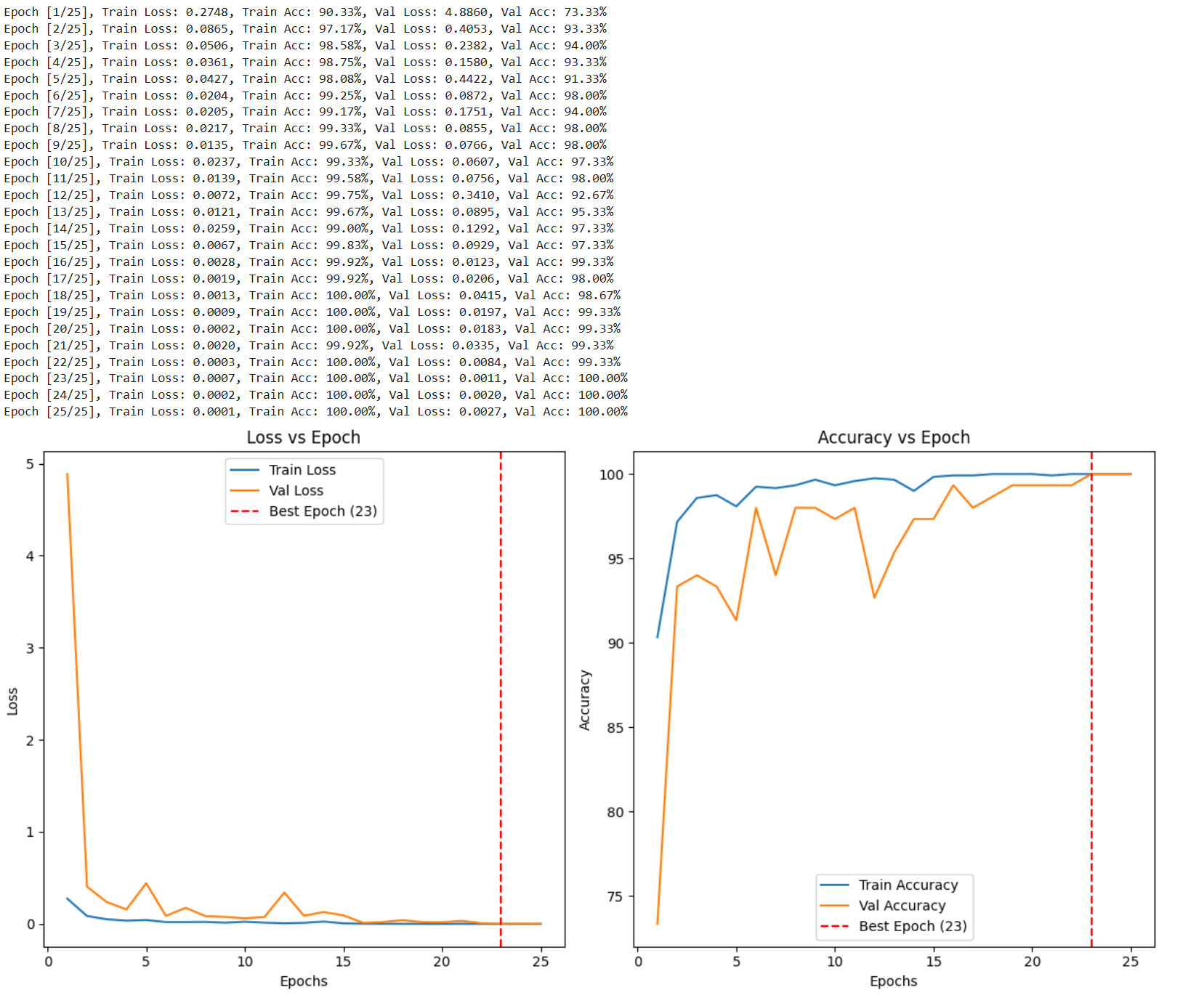

from sklearn.metrics import confusion_matrix, ConfusionMatrixDisplay
import matplotlib.pyplot as plt
import numpy as np

# Set model to evaluation mode
model.eval()

# Store all true and predicted labels
all_preds = []
all_labels = []

with torch.no_grad():
    for inputs, labels in testloader:  # or valloader
        inputs, labels = inputs.to(device), labels.to(device)
        outputs = model(inputs)
        _, preds = torch.max(outputs, 1)

        all_preds.extend(preds.cpu().numpy())
        all_labels.extend(labels.cpu().numpy())

# Get class names from the dataset
class_names = testloader.dataset.dataset.classes  # works with Subset or ImageFolder

# Compute confusion matrix
cm = confusion_matrix(all_labels, all_preds)
disp = ConfusionMatrixDisplay(confusion_matrix=cm, display_labels=class_names)

# Plot
fig, ax = plt.subplots(figsize=(10, 8))
disp.plot(cmap='Blues', ax=ax, xticks_rotation=45, values_format='d')
plt.title("Confusion Matrix with Crop Class Names")
plt.tight_layout()
plt.show()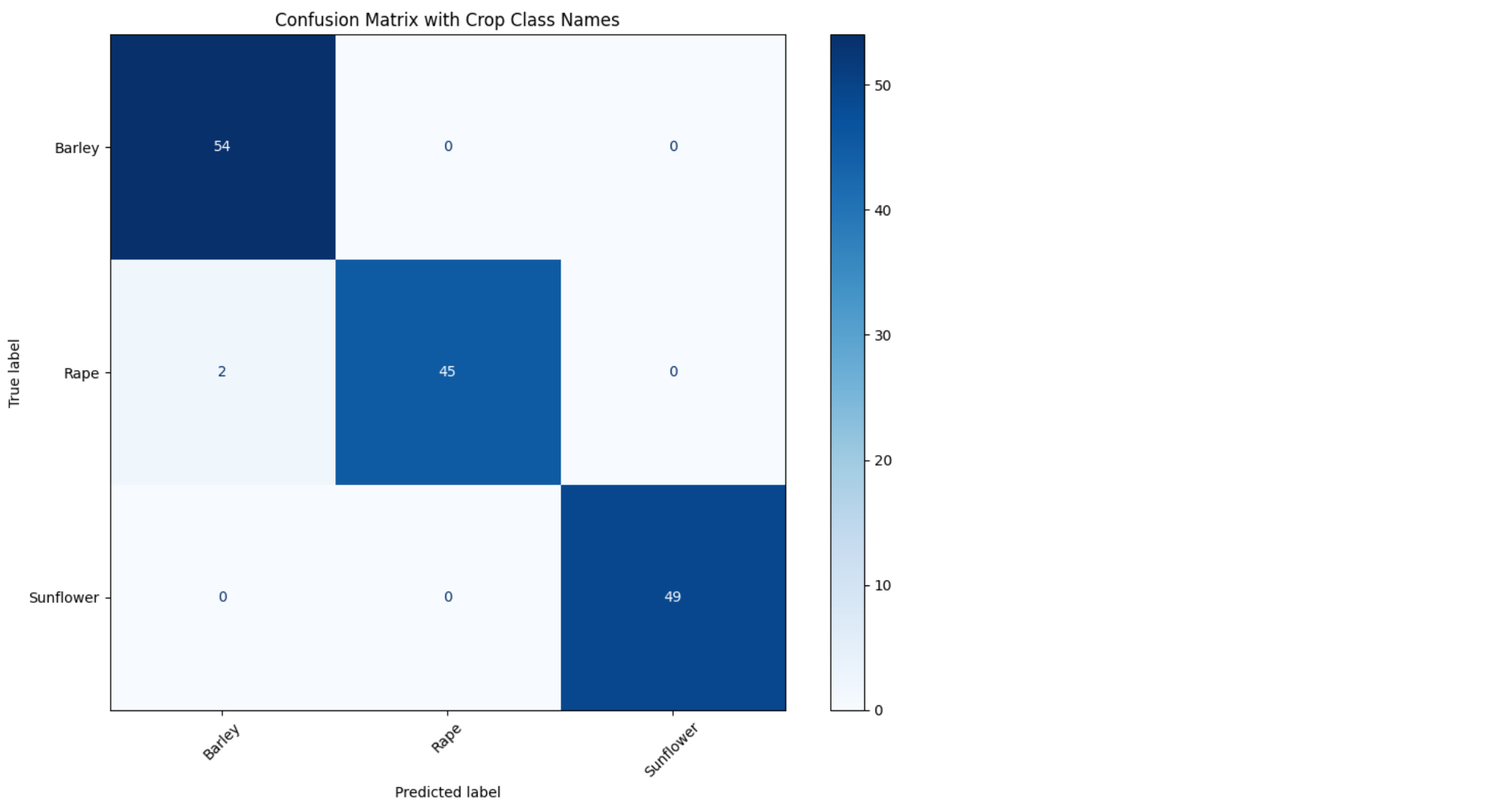

# Define the loss function
criterion = nn.CrossEntropyLoss()

# Function to evaluate accuracy and loss for a given dataloader
def evaluate_model(dataloader, dataset_name="dataset"):
    model.eval()
    total_loss = 0.0
    correct = 0
    total = 0

    with torch.no_grad():
        for images, labels in dataloader:
            images = images.to(device)
            labels = labels.to(device)

            # Forward pass
            outputs = model(images)
            loss = criterion(outputs, labels)

            # Accumulate loss
            total_loss += loss.item() * labels.size(0)  # Multiply by batch size to sum properly

            # Calculate accuracy
            _, predicted = torch.max(outputs.data, 1)
            total += labels.size(0)
            correct += (predicted == labels).sum().item()

    # Calculate mean loss and accuracy
    mean_loss = total_loss / total
    accuracy = 100 * correct / total

    print(f'Mean {dataset_name} loss: {mean_loss}')
    print(f'Accuracy of the model on the {dataset_name}: {accuracy} %')
    return mean_loss, accuracy

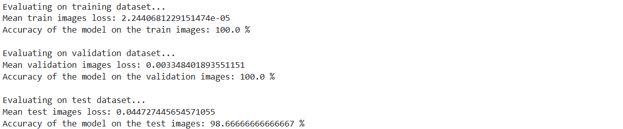
# Evaluate on the training dataset
print("Evaluating on training dataset...")
mean_train_loss, train_accuracy = evaluate_model(trainloader, dataset_name="train images")

# Evaluate on the validation dataset
print("\nEvaluating on validation dataset...")
mean_val_loss, val_accuracy = evaluate_model(valloader, dataset_name="validation images")

print("\nEvaluating on test dataset...")
mean_test_loss, test_accuracy = evaluate_model(testloader, dataset_name="test images")