Section 4
Self-Supervised Learning – SimCLR
Estimated Time: ~25 minutes
In this tutorial, we will train a SimCLR model using lightly. The model, augmentations and training procedure is from A Simple Framework for Contrastive Learning of Visual Representations.
The paper explores a rather simple training procedure for contrastive learning. Since we use the typical contrastive learning loss based on NCE the method greatly benefits from having larger batch sizes. In this example, we use a batch size of 256 and paired with the input resolution per image of 64x64 pixels and a resnet-18 model this example requires 16GB of GPU memory.
In this tutorial you will learn:
-
How to create a SimCLR model
-
How to generate image representations
-
How different augmentations impact the learned representations
Imports
Import the Python frameworks we need for this tutorial.
import os

import matplotlib.pyplot as plt
import numpy as np
import pytorch_lightning as pl
import torch
import torch.nn as nn
import torchvision
from PIL import Image
from sklearn.neighbors import NearestNeighbors
from sklearn.preprocessing import normalize

from lightly.data import LightlyDataset
from lightly.transforms import SimCLRTransform, utils
Configuration
We set some configuration parameters for our experiment. Feel free to change them and analyze the effect.
The default configuration with a batch size of 256 and input resolution of 128 requires 6GB of GPU memory.
# Configuration

num_workers = 8
batch_size = 256
seed = 1
max_epochs = 20
input_size = 128
num_ftrs = 32
Let's set the seed for our experiments
pl.seed_everything(seed)
path_to_data = "C:/Workshop/dataset_SL"Setup data augmentations and loaders
You can learn more about the different augmentations and learned invariances
here: lightly-advanced.
# Setup data augmentations and loaders
transform = SimCLRTransform(input_size=input_size, vf_prob=0.5, rr_prob=0.5)

# We create a torchvision transformation for embedding the dataset after
# training
test_transform = torchvision.transforms.Compose(
    [
        torchvision.transforms.Resize((input_size, input_size)),
        torchvision.transforms.ToTensor(),
        torchvision.transforms.Normalize(
            mean=utils.IMAGENET_NORMALIZE["mean"],
            std=utils.IMAGENET_NORMALIZE["std"],
        ),
    ]
)

dataset_train_simclr = LightlyDataset(input_dir=path_to_data, transform=transform)

dataset_test = LightlyDataset(input_dir=path_to_data, transform=test_transform)

dataloader_train_simclr = torch.utils.data.DataLoader(
    dataset_train_simclr,
    batch_size=batch_size,
    shuffle=True,
    drop_last=True,
    num_workers=num_workers,
)

dataloader_test = torch.utils.data.DataLoader(
    dataset_test,
    batch_size=batch_size,
    shuffle=False,
    drop_last=False,
    num_workers=num_workers,
)
Create the SimCLR Model
Now we create the SimCLR model. We implement it as a PyTorch Lightning Module
and use a ResNet-18 backbone from Torchvision. Lightly provides implementations
of the SimCLR projection head and loss function in the SimCLRProjectionHead
and NTXentLoss classes. We can simply import them and combine the building
blocks in the module.
# Create the SimCLR Model
from lightly.loss import NTXentLoss
from lightly.models.modules.heads import SimCLRProjectionHead

class SimCLRModel(pl.LightningModule):
    def __init__(self):
        super().__init__()

        # create a ResNet backbone and remove the classification head
        resnet = torchvision.models.resnet18()
        self.backbone = nn.Sequential(*list(resnet.children())[:-1])

        hidden_dim = resnet.fc.in_features
        self.projection_head = SimCLRProjectionHead(hidden_dim, hidden_dim, 128)

        self.criterion = NTXentLoss()

    def forward(self, x):
        h = self.backbone(x).flatten(start_dim=1)
        z = self.projection_head(h)
        return z

    def training_step(self, batch, batch_idx):
        (x0, x1), _, _ = batch
        z0 = self.forward(x0)
        z1 = self.forward(x1)
        loss = self.criterion(z0, z1)
        self.log("train_loss_ssl", loss)
        return loss

    def configure_optimizers(self):
        optim = torch.optim.SGD(
            self.parameters(), lr=6e-2, momentum=0.9, weight_decay=5e-4
        )
        scheduler = torch.optim.lr_scheduler.CosineAnnealingLR(optim, max_epochs)
        return [optim], [scheduler]
Train the module using the PyTorch Lightning Trainer on a single GPU.
model = SimCLRModel()
trainer = pl.Trainer(max_epochs=max_epochs, devices=1, accelerator="gpu")
trainer.fit(model, dataloader_train_simclr)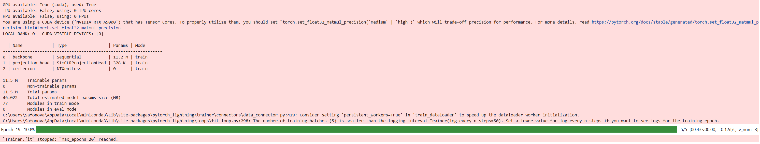
# Save the model's state_dict after training
torch.save(model.state_dict(), "simclr_pretrained_model.pth")
Next we create a helper function to generate embeddings from our test images using the model we just trained. Note that only the backbone is needed to generate embeddings, the projection head is only required for the training. Make sure to put the model into eval mode for this part!
# Next we create a helper function to generate embeddings from our test images using the model we just trained.
def generate_embeddings(model, dataloader):
    """Generates representations for all images in the dataloader with
    the given model
    """

    embeddings = []
    filenames = []
    with torch.no_grad():
        for img, _, fnames in dataloader:
            img = img.to(model.device)
            emb = model.backbone(img).flatten(start_dim=1)
            embeddings.append(emb)
            filenames.extend(fnames)

    embeddings = torch.cat(embeddings, 0)
    embeddings = normalize(embeddings)
    return embeddings, filenames

model.eval()
embeddings, filenames = generate_embeddings(model, dataloader_test)
Visualize Nearest Neighbors
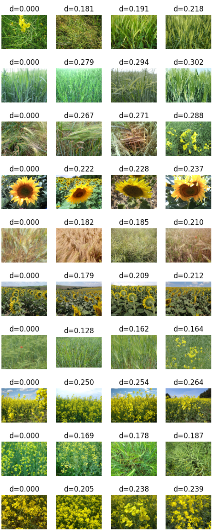
Let's look at the trained embedding and visualize the nearest neighbors for a few random samples.
We create some helper functions to simplify the work
def get_image_as_np_array(filename: str):
    """Returns an image as an numpy array"""
    img = Image.open(filename)
    return np.asarray(img)

def plot_knn_examples(embeddings, filenames, n_neighbors=4, num_examples=10):
    """Plots multiple rows of random images with their nearest neighbors"""
    # lets look at the nearest neighbors for some samples
    # we use the sklearn library
    nbrs = NearestNeighbors(n_neighbors=n_neighbors).fit(embeddings)
    distances, indices = nbrs.kneighbors(embeddings)

    # get 5 random samples
    samples_idx = np.random.choice(len(indices), size=num_examples, replace=False)

    # loop through our randomly picked samples
    for idx in samples_idx:
        fig = plt.figure()
        # loop through their nearest neighbors
        for plot_x_offset, neighbor_idx in enumerate(indices[idx]):
            # add the subplot
            ax = fig.add_subplot(1, len(indices[idx]), plot_x_offset + 1)
            # get the correponding filename for the current index
            fname = os.path.join(path_to_data, filenames[neighbor_idx])
            # plot the image
            plt.imshow(get_image_as_np_array(fname))
            # set the title to the distance of the neighbor
            ax.set_title(f"d={distances[idx][plot_x_offset]:.3f}")
            # let's disable the axis
            plt.axis("off")
plot_knn_examples(embeddings, filenames)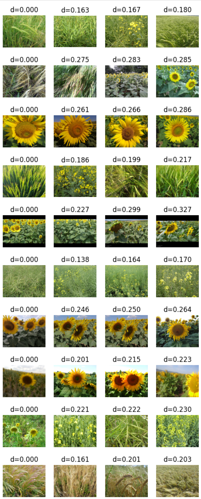
# Load the pretrained model
model = SimCLRModel()
model.load_state_dict(torch.load("simclr_pretrained_model.pth"))  # Load the pretrained weights
model.eval()  # Set the model to evaluation mode

# Generate embeddings using the pretrained model
embeddings, filenames = generate_embeddings(model, dataloader_test)
plot_knn_examples(embeddings, filenames)