Section 5
Self-Supervised Learning – SimSiam
Estimated Time: ~25 minutes
We will showcase how the generated embeddings can be used for exploration and better understanding of the raw data.
You can read up on the model in the paper Exploring Simple Siamese Representation Learning.
In this tutorial you will learn:
-
How to work with the SimSiam model
-
How to do self-supervised learning using PyTorch
-
How to check whether your embeddings have collapsed
# Import the Python frameworks

import math

import numpy as np
import torch
import torch.nn as nn
import torchvision

from lightly.data import LightlyDataset
from lightly.loss import NegativeCosineSimilarity
from lightly.models.modules.heads import SimSiamPredictionHead, SimSiamProjectionHead
from lightly.transforms import SimCLRTransform, utils
# seed torch and numpy
torch.manual_seed(0)
np.random.seed(0)
# set the path to the dataset
path_to_data = "C:/Workshop/dataset_SSL/train"Configuration
We set some configuration parameters for our experiment.
The default configuration with a batch size and input resolution of 256 requires 16GB of GPU memory.
num_workers = 8
batch_size = 128
seed = 1
epochs = 200
input_size = 256

# dimension of the embeddings
num_ftrs = 512
# dimension of the output of the prediction and projection heads
out_dim = proj_hidden_dim = 512
# the prediction head uses a bottleneck architecture
pred_hidden_dim = 128
Setup data augmentations and loaders
Since we're working with images, it makes sense to use horizontal and vertical flips as well as random rotation transformations. We apply weak color jitter to learn an invariance of the model with respect to slight changes in the color of the water.
# define the augmentations for self-supervised learning
transform = SimCLRTransform(
    input_size=input_size,
    # require invariance to flips and rotations
    hf_prob=0.5,
    vf_prob=0.5,
    rr_prob=0.5,
    # satellite images are all taken from the same height
    # so we use only slight random cropping
    min_scale=0.5,
    # use a weak color jitter for invariance w.r.t small color changes
    cj_prob=0.2,
    cj_bright=0.1,
    cj_contrast=0.1,
    cj_hue=0.1,
    cj_sat=0.1,
)

# create a lightly dataset for training with augmentations
dataset_train_simsiam = LightlyDataset(input_dir=path_to_data, transform=transform)

# create a dataloader for training
dataloader_train_simsiam = torch.utils.data.DataLoader(
    dataset_train_simsiam,
    batch_size=batch_size,
    shuffle=True,
    drop_last=True,
    num_workers=num_workers,
)

# create a torchvision transformation for embedding the dataset after training
# here, we resize the images to match the input size during training and apply
# a normalization of the color channel based on statistics from imagenet
test_transforms = torchvision.transforms.Compose(
    [
        torchvision.transforms.Resize((input_size, input_size)),
        torchvision.transforms.ToTensor(),
        torchvision.transforms.Normalize(
            mean=utils.IMAGENET_NORMALIZE["mean"],
            std=utils.IMAGENET_NORMALIZE["std"],
        ),
    ]
)

# create a lightly dataset for embedding
dataset_test = LightlyDataset(input_dir=path_to_data, transform=test_transforms)

# create a dataloader for embedding
dataloader_test = torch.utils.data.DataLoader(
    dataset_test,
    batch_size=batch_size,
    shuffle=False,
    drop_last=False,
    num_workers=num_workers,
)
Create the SimSiam model
Create a ResNet backbone and remove the classification head
class SimSiam(nn.Module):
    def __init__(self, backbone, num_ftrs, proj_hidden_dim, pred_hidden_dim, out_dim):
        super().__init__()
        self.backbone = backbone
        self.projection_head = SimSiamProjectionHead(num_ftrs, proj_hidden_dim, out_dim)
        self.prediction_head = SimSiamPredictionHead(out_dim, pred_hidden_dim, out_dim)

    def forward(self, x):
        # get representations
        f = self.backbone(x).flatten(start_dim=1)
        # get projections
        z = self.projection_head(f)
        # get predictions
        p = self.prediction_head(z)
        # stop gradient
        z = z.detach()
        return z, p

# we use a pretrained resnet for this tutorial to speed
# up training time but you can also train one from scratch
resnet = torchvision.models.resnet18()
backbone = nn.Sequential(*list(resnet.children())[:-1])
model = SimSiam(backbone, num_ftrs, proj_hidden_dim, pred_hidden_dim, out_dim)
SimSiam uses a symmetric negative cosine similarity loss and does therefore not require any negative samples. We build a criterion and an optimizer.
# SimSiam uses a symmetric negative cosine similarity loss
criterion = NegativeCosineSimilarity()

# scale the learning rate
lr = 0.05 * batch_size / 256
# use SGD with momentum and weight decay
optimizer = torch.optim.SGD(model.parameters(), lr=lr, momentum=0.9, weight_decay=5e-4)
Train SimSiam
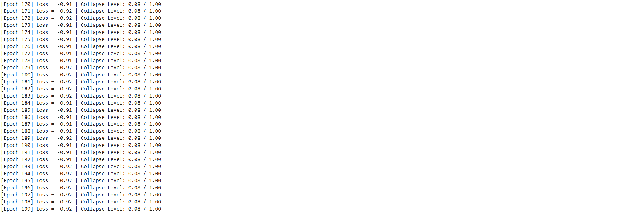
To train the SimSiam model, you can use a classic PyTorch training loop: For every epoch, iterate over all batches in the training data, extract the two transforms of every image, pass them through the model, and calculate the loss. Then, simply update the weights with the optimizer. Don't forget to reset the gradients!
Since SimSiam doesn't require negative samples, it is a good idea to check whether the outputs of the model have collapsed into a single direction. For this we can simply check the standard deviation of the L2 normalized output vectors. If it is close to one divided by the square root of the output dimension, everything is fine (you can read up on this idea here).
device = "cuda" if torch.cuda.is_available() else "cpu"
model.to(device)
avg_loss = 0.0
avg_output_std = 0.0
for e in range(epochs):
for (x0, x1), _, _ in dataloader_train_simsiam:
# move images to the gpu
x0 = x0.to(device)
x1 = x1.to(device)
# run the model on both transforms of the images
# we get projections (z0 and z1) and
# predictions (p0 and p1) as output
z0, p0 = model(x0)
z1, p1 = model(x1)
# apply the symmetric negative cosine similarity
# and run backpropagation
loss = 0.5 * (criterion(z0, p1) + criterion(z1, p0))
loss.backward()
optimizer.step()
optimizer.zero_grad()
# calculate the per-dimension standard deviation of the outputs
# we can use this later to check whether the embeddings are collapsing
output = p0.detach()
output = torch.nn.functional.normalize(output, dim=1)
output_std = torch.std(output, 0)
output_std = output_std.mean()
# use moving averages to track the loss and standard deviation
w = 0.9
avg_loss = w * avg_loss + (1 - w) * loss.item()
avg_output_std = w * avg_output_std + (1 - w) * output_std.item()
# the level of collapse is large if the standard deviation of the l2
# normalized output is much smaller than 1 / sqrt(dim)
collapse_level = max(0.0, 1 - math.sqrt(out_dim) * avg_output_std)
# print intermediate results
print(
f"[Epoch {e:3d}] "
f"Loss = {avg_loss:.2f} | "
f"Collapse Level: {collapse_level:.2f} / 1.00"
)
# Save the model's state dict (weights)
torch.save(model.state_dict(), "simsiam_pretrained_model.pth")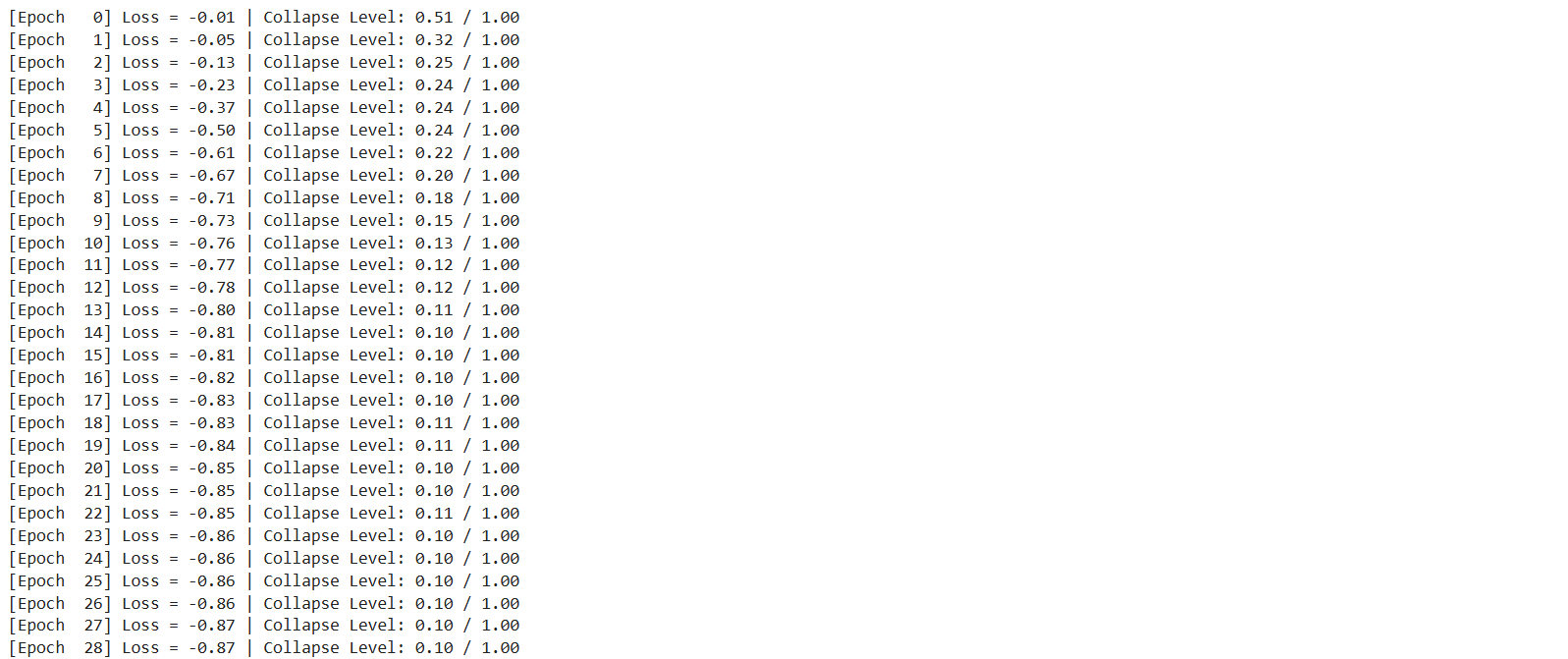 ...
...
embeddings = []
filenames = []

# disable gradients for faster calculations
model.eval()
with torch.no_grad():
    for i, (x, _, fnames) in enumerate(dataloader_test):
        # move the images to the gpu
        x = x.to(device)
        # embed the images with the pre-trained backbone
        y = model.backbone(x).flatten(start_dim=1)
        # store the embeddings and filenames in lists
        embeddings.append(y)
        filenames = filenames + list(fnames)

# concatenate the embeddings and convert to numpy
embeddings = torch.cat(embeddings, dim=0)
embeddings = embeddings.cpu().numpy()
Scatter Plot and Nearest Neighbors
Now that we have the embeddings, we can visualize the data with a scatter plot. Further down, we also check out the nearest neighbors of a few example images.
As a first step, we make a few additional imports.
# for plotting
import os

import matplotlib.offsetbox as osb
import matplotlib.pyplot as plt

# for resizing images to thumbnails
import torchvision.transforms.functional as functional
from matplotlib import rcParams as rcp
from PIL import Image

# for clustering and 2d representations
from sklearn import random_projection
Then, we transform the embeddings using UMAP and rescale them to fit in the [0, 1] square.
# for the scatter plot we want to transform the images to a two-dimensional
# vector space using a random Gaussian projection
projection = random_projection.GaussianRandomProjection(n_components=2)
embeddings_2d = projection.fit_transform(embeddings)

# normalize the embeddings to fit in the [0, 1] square
M = np.max(embeddings_2d, axis=0)
m = np.min(embeddings_2d, axis=0)
embeddings_2d = (embeddings_2d - m) / (M - m)
Let's start with a nice scatter plot of our dataset! The helper function below will create one.
def get_scatter_plot_with_thumbnails():
    """Creates a scatter plot with image overlays."""
    # initialize empty figure and add subplot
    fig = plt.figure()
    fig.suptitle("Scatter Plot of the Sentinel-2 Dataset")
    ax = fig.add_subplot(1, 1, 1)
    # shuffle images and find out which images to show
    shown_images_idx = []
    shown_images = np.array([[1.0, 1.0]])
    iterator = [i for i in range(embeddings_2d.shape[0])]
    np.random.shuffle(iterator)
    for i in iterator:
        # only show image if it is sufficiently far away from the others
        dist = np.sum((embeddings_2d[i] - shown_images) ** 2, 1)
        if np.min(dist) < 2e-3:
            continue
        shown_images = np.r_[shown_images, [embeddings_2d[i]]]
        shown_images_idx.append(i)

    # plot image overlays
    for idx in shown_images_idx:
        thumbnail_size = int(rcp["figure.figsize"][0] * 2.0)
        path = os.path.join(path_to_data, filenames[idx])
        img = Image.open(path)
        img = functional.resize(img, thumbnail_size)
        img = np.array(img)
        img_box = osb.AnnotationBbox(
            osb.OffsetImage(img, cmap=plt.cm.gray_r),
            embeddings_2d[idx],
            pad=0.2,
        )
        ax.add_artist(img_box)

    # set aspect ratio
    ratio = 1.0 / ax.get_data_ratio()
    ax.set_aspect(ratio, adjustable="box")

# get a scatter plot with thumbnail overlays
get_scatter_plot_with_thumbnails()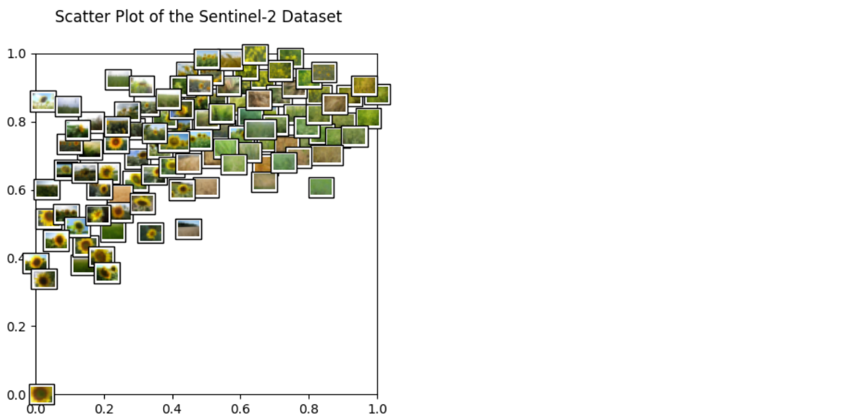
Next, we plot example images and their nearest neighbors (calculated from the embeddings generated above). This is a very simple approach to find more images of a certain type where a few examples are already available. For example, when a subset of the data is already labelled and one class of images is clearly underrepresented, one can easily query more images of this class from the unlabelled dataset.
Let's get to work! The plots are shown below.
example_images = [
    "202257442466LCLU_CropLC1.jpg",  # Barley
    "LUCAS2006_46182994_Cover.jpg",  # Rape
    "LUCAS2009_46442776_Cover.jpg",  # Sunflower
]

def get_image_as_np_array(filename: str):
    """Loads the image with filename and returns it as a numpy array."""
    img = Image.open(filename)
    return np.asarray(img)

def get_image_as_np_array_with_frame(filename: str, w: int = 5):
    """Returns an image as a numpy array with a black frame of width w."""
    img = get_image_as_np_array(filename)
    ny, nx, _ = img.shape
    # create an empty image with padding for the frame
    framed_img = np.zeros((w + ny + w, w + nx + w, 3))
    framed_img = framed_img.astype(np.uint8)
    # put the original image in the middle of the new one
    framed_img[w:-w, w:-w] = img
    return framed_img

def plot_nearest_neighbors_3x3(example_image: str, i: int):
    """Plots the example image and its eight nearest neighbors."""
    n_subplots = 9
    # initialize empty figure
    fig = plt.figure()
    fig.suptitle(f"Nearest Neighbor Plot {i + 1}")
    #
    example_idx = filenames.index(example_image)
    # get distances to the cluster center
    distances = embeddings - embeddings[example_idx]
    distances = np.power(distances, 2).sum(-1).squeeze()
    # sort indices by distance to the center
    nearest_neighbors = np.argsort(distances)[:n_subplots]
    # show images
    for plot_offset, plot_idx in enumerate(nearest_neighbors):
        ax = fig.add_subplot(3, 3, plot_offset + 1)
        # get the corresponding filename
        fname = os.path.join(path_to_data, filenames[plot_idx])
        if plot_offset == 0:
            ax.set_title(f"Example Image")
            plt.imshow(get_image_as_np_array_with_frame(fname))
        else:
            plt.imshow(get_image_as_np_array(fname))
        # let's disable the axis
        plt.axis("off")

# show example images for each cluster
for i, example_image in enumerate(example_images):
    plot_nearest_neighbors_3x3(example_image, i)